Download this example as Julia file or Jupyter notebook.
8. Momentum transfer conventions
Sunny defines the dynamical structure factor following conventions as in Squire and Boothroyd,
\[\mathcal{S}^{αβ}(𝐪, ω) ≡ \frac{1}{2π} \int_{-∞}^{∞} e^{-iωt} ⟨\hat{M}^{†α}_𝐪(0) \hat{M}^β_𝐪(t)⟩ dt.\]
The momentum-space dipole operator $\hat{𝐌}_𝐪$ is obtained from the real-space density $\hat{𝐌}(𝐫)$ using the Fourier transform convention,
\[\hat{𝐌}_𝐪 ≡ \int_V e^{+ i 𝐪⋅𝐫} \hat{𝐌}(𝐫) d𝐫.\]
With appropriate contraction of spin components, $\mathcal{S}^{αβ}(𝐪, ω)$ directly relates to the neutron scattering cross-section. Here, $𝐪$ and $ω$ represent momentum and energy transfer to the sample. Sunny will report the structure factor as an intensive quantity by dividing by the number of chemical cells in the macroscopic sample. Full details are given in the documentation page Structure Factor Conventions.
If the spin Hamiltonian lacks inversion symmetry, intensities at $±𝐪$ may be inequivalent. A simple example is the 1D chain with competing Ising and Dzyaloshinskii–Moriya couplings. Sunny calculations on this model can be compared to those of other codes. For example, SpinW employs the opposite sign convention for the momentum transfer $𝐪$.
1D model lacking reflection symmetry
using Sunny, GLMakieCreate a Crystal with spacegroup P1 to effectively disable all symmetry analysis. This avoids any symmetry-imposed constraints on the couplings. Because all bonds are treated as symmetry-inequivalent, each coupling must be specified independently; there is no automatic propagation to "equivalent" bonds.
latvecs = lattice_vectors(1, 1, 1, 90, 90, 90)
cryst = Crystal(latvecs, [[0, 0, 0]], "P1")
Crystal
Spacegroup 'P 1' (1)
Lattice params a=1, b=1, c=1, α=90°, β=90°, γ=90°
Cell volume 1
Wyckoff 1a (site sym. '1'):
1. [0, 0, 0]
Include DM and Ising couplings between nearest neighbors on a chain. Letting $j$ denote the site position along axis $𝐚_3$, the full Hamiltonian is
\[ℋ = 𝐃 ⋅ ∑_j 𝐒_j × 𝐒_{j+1} - J ∑_j ∑_j S^z_j S^z_{j+1},\]
with dmvec $𝐃 = D ẑ$.
s = 3/2
sys = System(cryst, [1 => Moment(; s, g=2)], :dipole)
J = 1.0
D = 0.2
z = [0, 0, 1]
set_exchange!(sys, dmvec(D * z) - J * z * z', Bond(1, 1, [0, 0, 1]))
The relatively large Ising coupling favors one of two polarized states, $±ẑ$. Use polarize_spins! to align $𝐒$ with $+ẑ$. This polarization could also be realized via an applied $𝐁$ field in the opposite direction, as documented in set_field!.
polarize_spins!(sys, [0, 0, 1])
@assert energy(sys) ≈ - s^2
plot_spins(sys)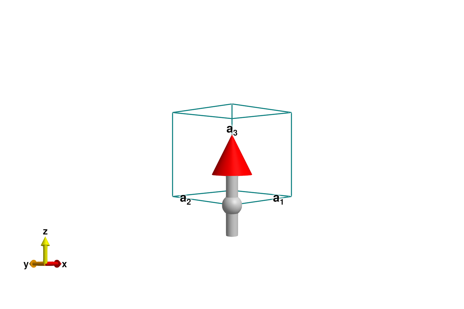
Intensities from linear spin wave theory
The SpinWaveTheory calculation shows a single band with dispersion $ϵ(𝐪) = 2 s [J ± D \sin(2πq_3)]$ for the polarization state $𝐒 = ± s ẑ$. There is a clear dependence on the sign of $q_3$.
path = q_space_path(cryst, [[0, 0, -1/2], [0, 0, 0], [0, 0, +1/2]], 400)
swt = SpinWaveTheory(sys; measure=ssf_trace(sys))
res = intensities_bands(swt, path)
plot_intensities(res; ylims=(0, 5))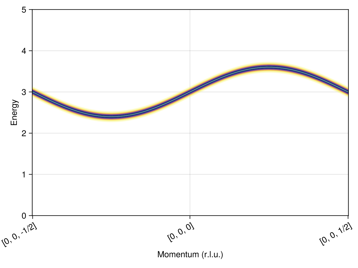
Intensities from classical spin dynamics
Classical dynamics at low temperatures produces, in principle, the same excitation spectrum. Here, finite-size effects will limit $𝐪$-space resolution. Use resize_supercell to study a chain of 32 sites.
sys2 = resize_supercell(sys, (1, 1, 32))System [Dipole mode]
Supercell (1×1×32)×1
Energy per site -9/4
Use Langevin dynamics to sample from the classical Boltzmann distribution at a relatively low temperature, $k_B T / J = 0.03$
dt = 0.03 / J
kT = 0.03 * J
damping = 0.1
langevin = Langevin(dt; kT, damping)
suggest_timestep(sys2, langevin; tol=1e-2)
for _ in 1:10_000
    step!(sys, langevin)
end
Consider dt ≈ 0.03296 for this spin configuration at tol = 0.01000. Current value is dt = 0.03000.Use SampledCorrelations to collect statistics from classical spin dynamic trajectories.
sc = SampledCorrelations(sys2; dt, energies=range(0, 5, 100), measure=ssf_trace(sys2))
add_sample!(sc, sys2)
nsamples = 100
for _ in 1:nsamples
for _ in 1:1000
step!(sys2, langevin)
end
add_sample!(sc, sys2)
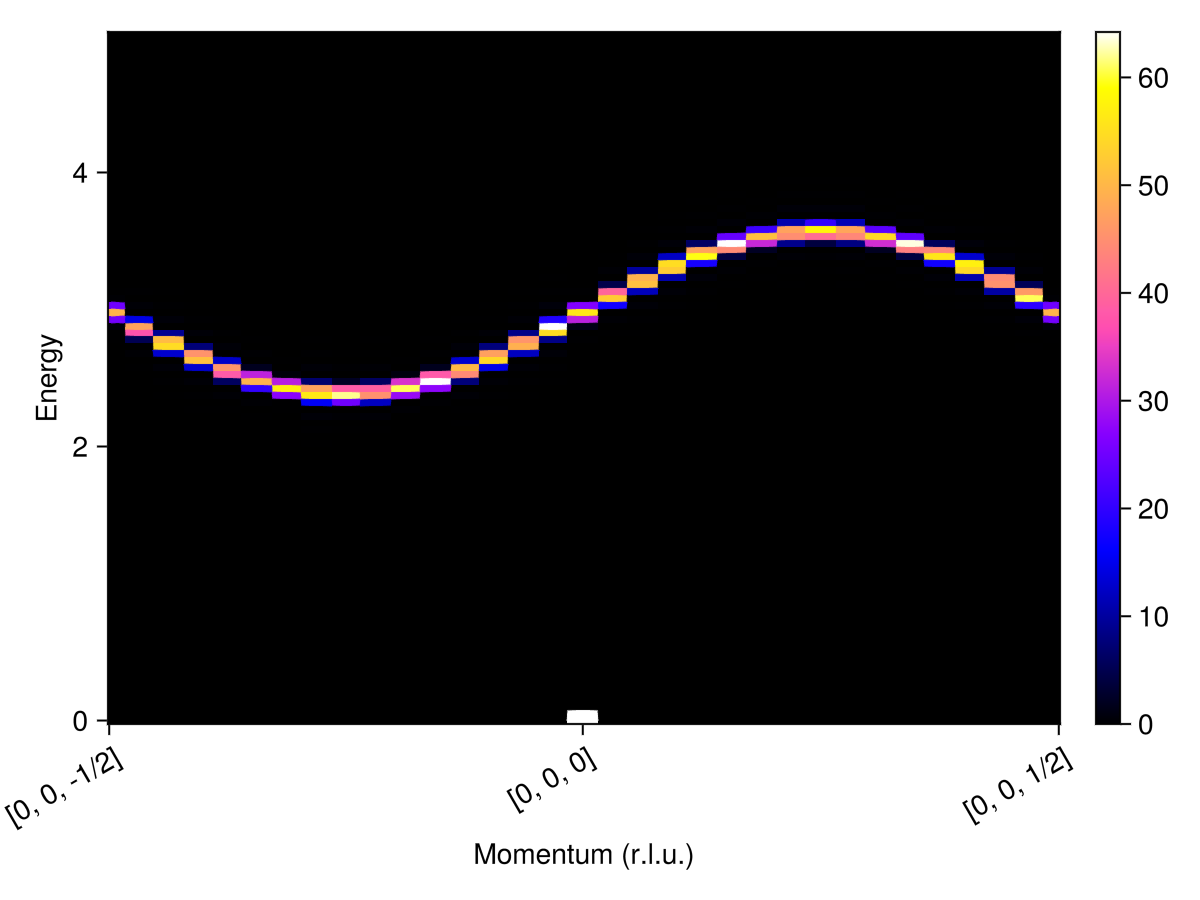
endIn the limit $T → 0$, the intensities match linear spin wave theory up to finite-size effects and statistical error. Additionally, the classical dynamics calculation shows the elastic peak at $𝐪 = [0,0,0]$, associated with the ferromagnetic ground state.
res2 = intensities(sc, path; energies=:available, kT)
plot_intensities(res2)