Download this example as Jupyter notebook or Julia script.

2. Spin wave simulations of CoRh₂O₄

This tutorial illustrates the conventional spin wave theory of dipoles. We consider a simple model of the diamond-cubic crystal CoRh₂O₄, with parameters extracted from Ge et al., Phys. Rev. B 96, 064413.

using Sunny, GLMakie

Construct a diamond Crystal in the conventional (non-primitive) cubic unit cell. Sunny will populate all eight symmetry-equivalent sites when given the international spacegroup number 227 ("Fd-3m") and the appropriate setting. For this spacegroup, there are two conventional translations of the unit cell, and it is necessary to disambiguate through the setting keyword argument. (On your own: what happens if setting is omitted?)

a = 8.5031 # (Å)
latvecs = lattice_vectors(a, a, a, 90, 90, 90)
cryst = Crystal(latvecs, [[0,0,0]], 227, setting="1")

Crystal
Spacegroup 'F d -3 m' (227)
Lattice params a=8.503, b=8.503, c=8.503, α=90°, β=90°, γ=90°
Cell volume 614.8
Wyckoff 8a (point group '-43m'):
   1. [0, 0, 0]
   2. [1/2, 1/2, 0]
   3. [1/4, 1/4, 1/4]
   4. [3/4, 3/4, 1/4]
   5. [1/2, 0, 1/2]
   6. [0, 1/2, 1/2]
   7. [3/4, 1/4, 3/4]
   8. [1/4, 3/4, 3/4]

In a running Julia environment, the crystal can be viewed interactively using view_crystal.

view_crystal(cryst)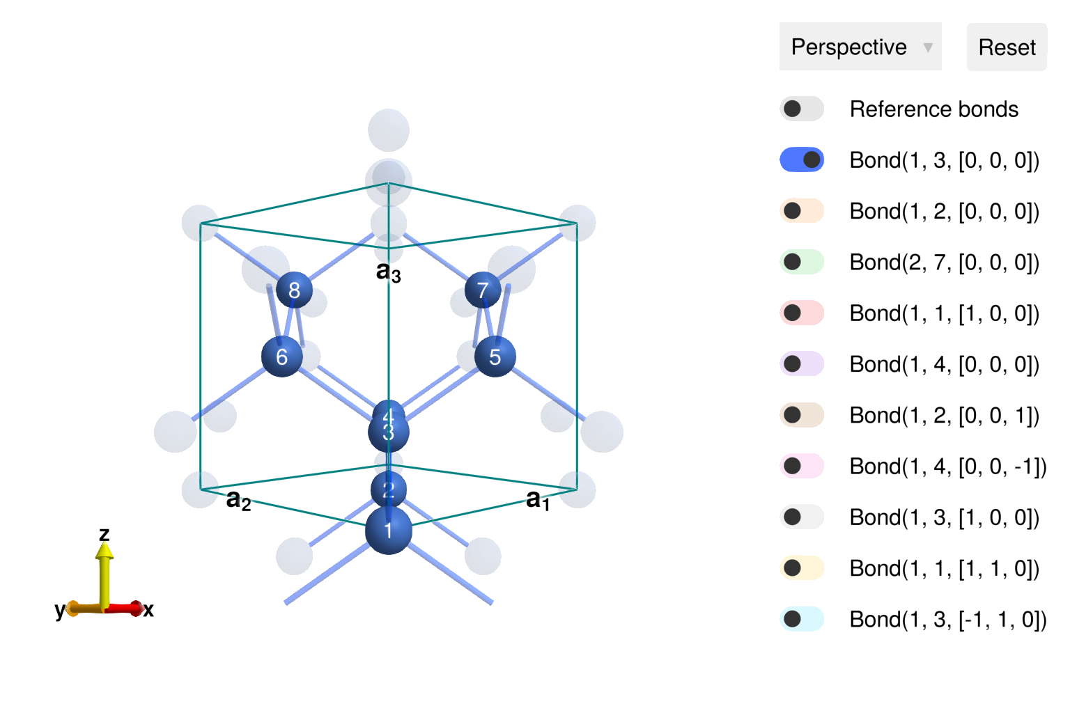

Construct a System with quantum spin $S=3/2$ constrained to the space of dipoles. Including an antiferromagnetic nearest neighbor interaction J will favor Néel order. To optimize this magnetic structure, it is sufficient to employ a magnetic lattice consisting of a single crystal unit cell, latsize=(1,1,1). Passing an explicit random number seed will ensure repeatable results.

latsize = (1, 1, 1)
S = 3/2
J = 0.63 # (meV)
sys = System(cryst, latsize, [SpinInfo(1; S, g=2)], :dipole; seed=0)
set_exchange!(sys, J, Bond(1, 3, [0,0,0]))

In the ground state, each spin is exactly anti-aligned with its 4 nearest-neighbors. Because every bond contributes an energy of $-JS^2$, the energy per site is $-2JS^2$. In this calculation, a factor of 1/2 avoids double-counting the bonds. Due to lack of frustration, direct energy minimization is successful in finding the ground state.

randomize_spins!(sys)
minimize_energy!(sys)

@assert energy_per_site(sys) ≈ -2J*S^2

Plotting the spins confirms the expected Néel order. Note that the overall, global rotation of dipoles is arbitrary.

s0 = sys.dipoles[1,1,1,1]
plot_spins(sys; color=[s'*s0 for s in sys.dipoles])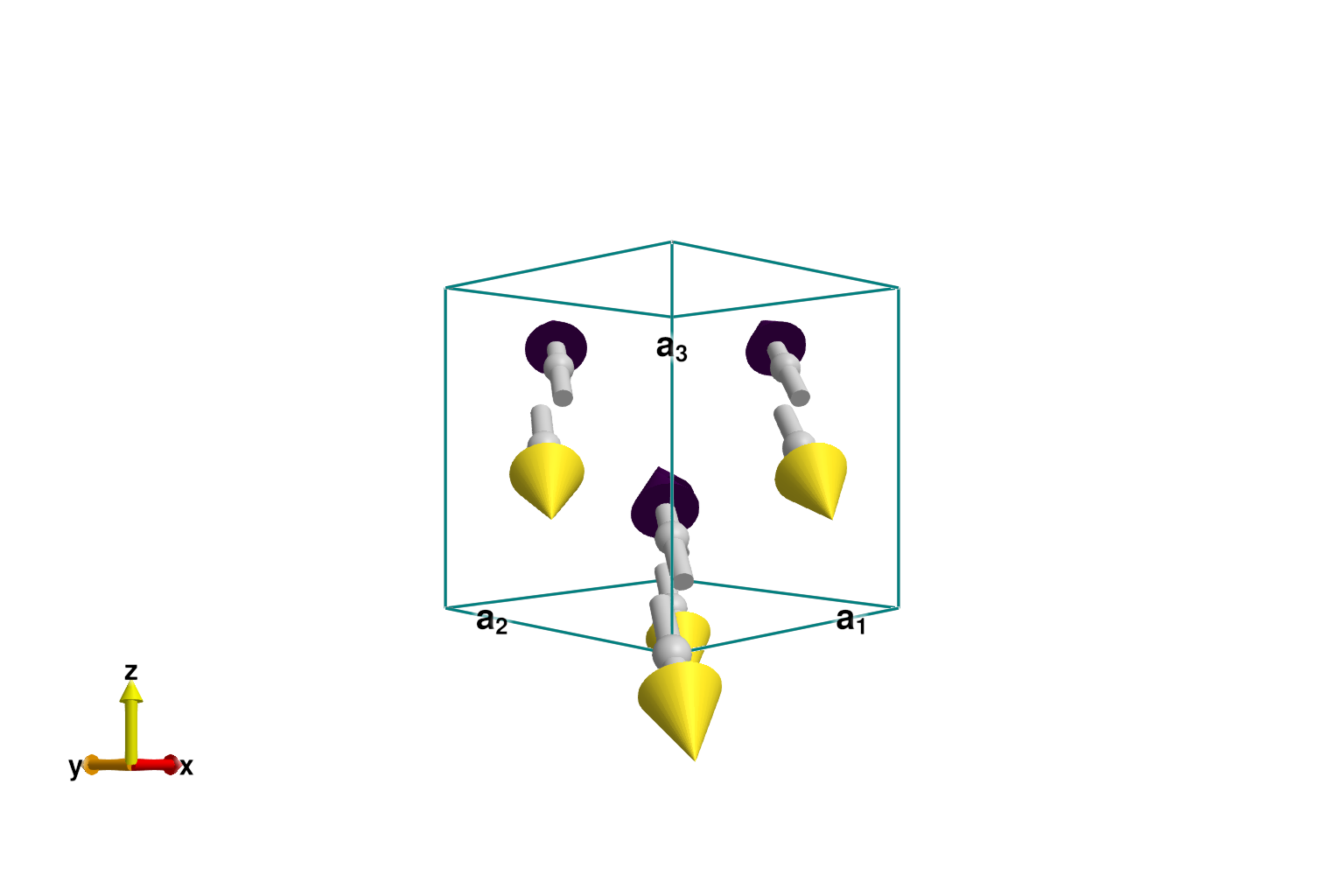

For numerical efficiency, it is helpful to work with the smallest possible magnetic supercell; in this case, it is the primitive cell. The columns of the 3×3 shape matrix define the lattice vectors of the primitive cell as multiples of the conventional, cubic lattice vectors. After transforming the system with reshape_supercell, the energy per site remains the same.

shape = [0 1 1;
         1 0 1;
         1 1 0] / 2
sys_prim = reshape_supercell(sys, shape)
@assert energy_per_site(sys_prim) ≈ -2J*S^2
plot_spins(sys_prim; color=[s'*s0 for s in sys_prim.dipoles])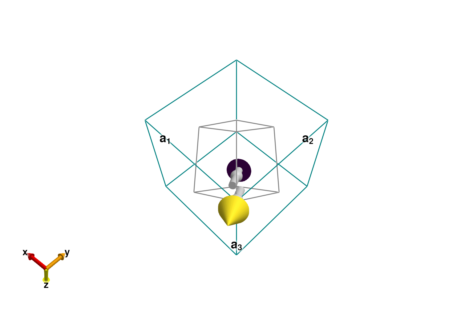

Now estimate $𝒮(𝐪,ω)$ with SpinWaveTheory and an intensity_formula. The mode :perp contracts with a dipole factor to return the unpolarized intensity. The formula also employs lorentzian broadening. The isotropic FormFactor for Cobalt(2+) dampens intensities at large $𝐪$.

swt = SpinWaveTheory(sys_prim)
kernel = lorentzian(fwhm=0.8)
formfactors = [FormFactor("Co2")]
formula = intensity_formula(swt, :perp; kernel, formfactors)

Quantum Scattering Intensity Formula
At any (Q,ω), with S = S(Q,ωᵢ):

  Intensity(Q,ω) = ∑ᵢ Kernel(ω-ωᵢ) ∑_ij (I - Q⊗Q){i,j} S{i,j}
                                   
                                   (i,j = Sx,Sy,Sz)

Intensity(ω) reported

For the "single crystal" result, we may use reciprocal_space_path to construct a path that connects high-symmetry points in reciprocal space. The intensities_broadened function collects intensities along this path for the given set of energy values.

qpoints = [[0, 0, 0], [1/2, 0, 0], [1/2, 1/2, 0], [0, 0, 0]]
path, xticks = reciprocal_space_path(cryst, qpoints, 50)
energies = collect(0:0.01:6)
is = intensities_broadened(swt, path, energies, formula)

fig = Figure()
ax = Axis(fig[1,1]; aspect=1.4, ylabel="ω (meV)", xlabel="𝐪 (r.l.u.)",
          xticks, xticklabelrotation=π/10)
heatmap!(ax, 1:size(is, 1), energies, is, colormap=:gnuplot2)
fig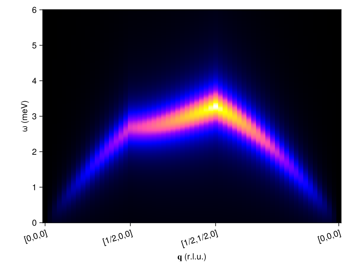

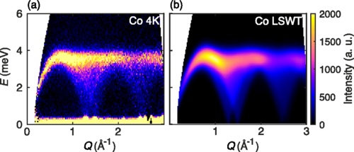
A powder measurement effectively involves an average over all possible crystal orientations. We use the function reciprocal_space_shell to sample n wavevectors on a sphere of a given radius (inverse angstroms), and then calculate the spherically-averaged intensity.

radii = 0.01:0.02:3 # (1/Å)
output = zeros(Float64, length(radii), length(energies))
for (i, radius) in enumerate(radii)
    n = 300
    qs = reciprocal_space_shell(cryst, radius, n)
    is = intensities_broadened(swt, qs, energies, formula)
    output[i, :] = sum(is, dims=1) / size(is, 1)
end

fig = Figure()
ax = Axis(fig[1,1]; xlabel="Q (Å⁻¹)", ylabel="ω (meV)")
heatmap!(ax, radii, energies, output, colormap=:gnuplot2)
fig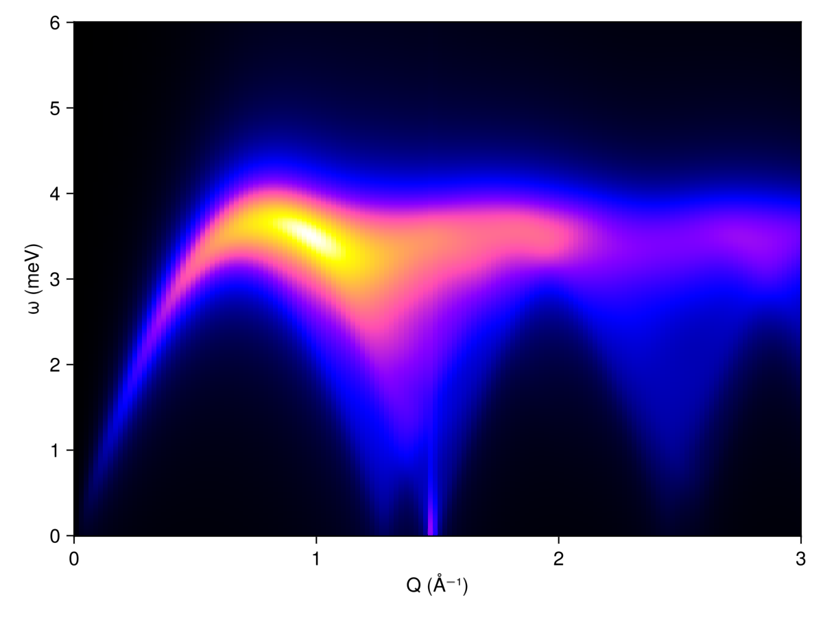

This result can be compared to experimental neutron scattering data from Fig. 5 of Ge et al.