Download this example as Jupyter notebook or Julia script.

3. Landau-Lifshitz dynamics of CoRh₂O₄ at finite T

using Sunny, GLMakie, Statistics

System construction

Construct the system as in the previous CoRh₂O₄ tutorial. After optimization, the system will be in an unfrustrated antiferromagnetic ground state.

a = 8.5031 # (Å)
latvecs = lattice_vectors(a, a, a, 90, 90, 90)
cryst = Crystal(latvecs, [[0,0,0]], 227, setting="1")

units = Units(:meV)
latsize = (2, 2, 2)
S = 3/2
J = 0.63 # (meV)
sys = System(cryst, latsize, [SpinInfo(1; S, g=2)], :dipole; seed=0)
set_exchange!(sys, J, Bond(1, 3, [0,0,0]))
randomize_spins!(sys)
minimize_energy!(sys)

Use resize_supercell to build a new system with a lattice of 10×10×10 unit cells. The desired Néel order is retained.

sys = resize_supercell(sys, (10, 10, 10))
@assert energy_per_site(sys) ≈ -2J*S^2

We will be using a Langevin spin dynamics to thermalize the system. This dynamics involves a dimensionless damping magnitude and target temperature kT for thermal fluctuations.

kT = 16 * units.K  # 16 K ≈ 1.38 meV, slightly below ordering temperature
langevin = Langevin(; damping=0.2, kT)

Langevin(<missing>; damping=0.2, kT=1.3787733219432283)

Use suggest_timestep to select an integration timestep for the given error tolerance, e.g. tol=1e-2. The spin configuration in sys should ideally be relaxed into thermal equilibrium, but the current, energy-minimized configuration will also work reasonably well.

suggest_timestep(sys, langevin; tol=1e-2)
langevin.dt = 0.025;

Consider dt ≈ 0.02528 for this spin configuration at tol = 0.01.

Now run a dynamical trajectory to sample spin configurations. Keep track of the energy per site at each time step.

energies = [energy_per_site(sys)]
for _ in 1:1000
    step!(sys, langevin)
    push!(energies, energy_per_site(sys))
end

Now that the spin configuration has relaxed, we can learn that dt was a little smaller than necessary; increasing it will make the remaining simulations faster.

suggest_timestep(sys, langevin; tol=1e-2)
langevin.dt = 0.042;

Consider dt ≈ 0.04209 for this spin configuration at tol = 0.01. Current value is dt = 0.025.

The energy per site has converged, which suggests that the system has reached thermal equilibrium.

plot(energies, color=:blue, figure=(size=(600,300),), axis=(xlabel="Timesteps", ylabel="Energy (meV)"))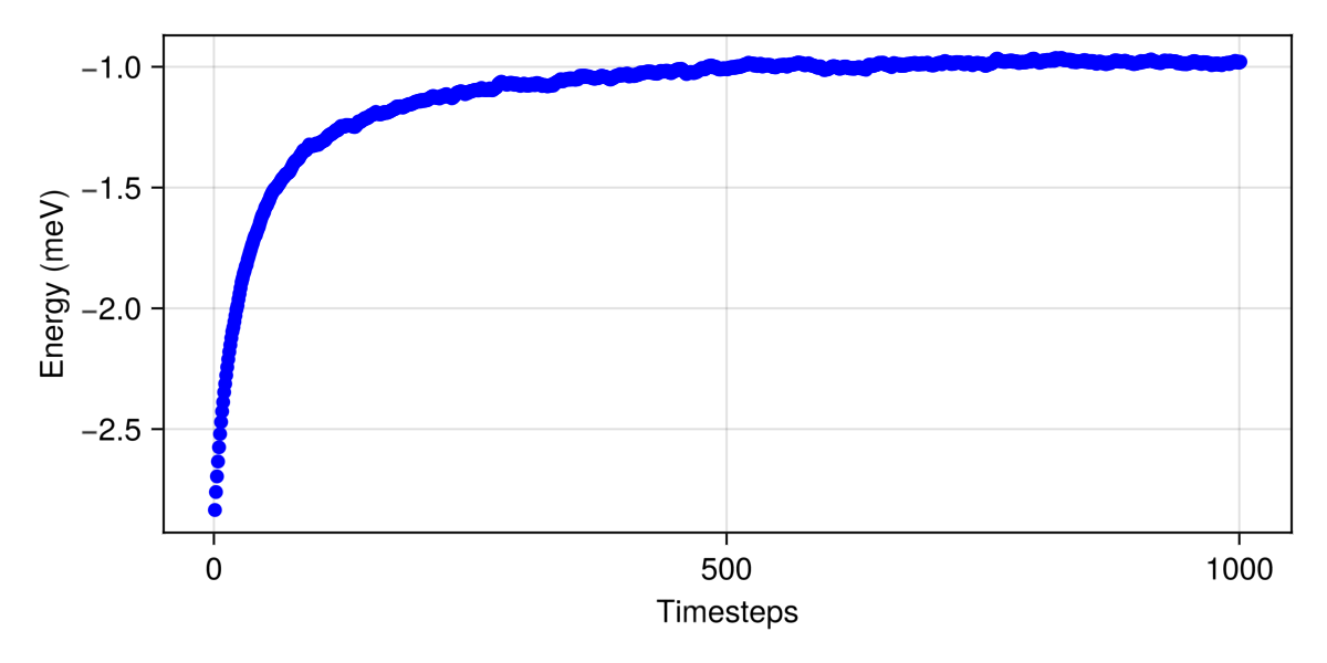

Thermal fluctuations are apparent in the spin configuration.

S_ref = sys.dipoles[1,1,1,1]
plot_spins(sys; color=[s'*S_ref for s in sys.dipoles])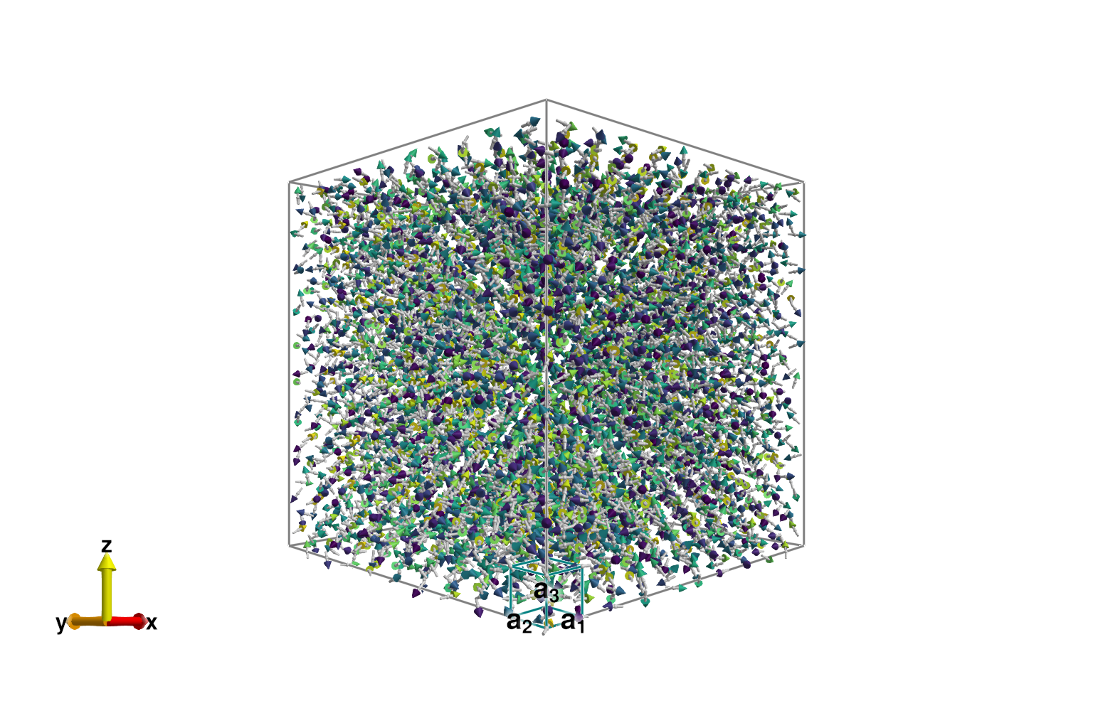

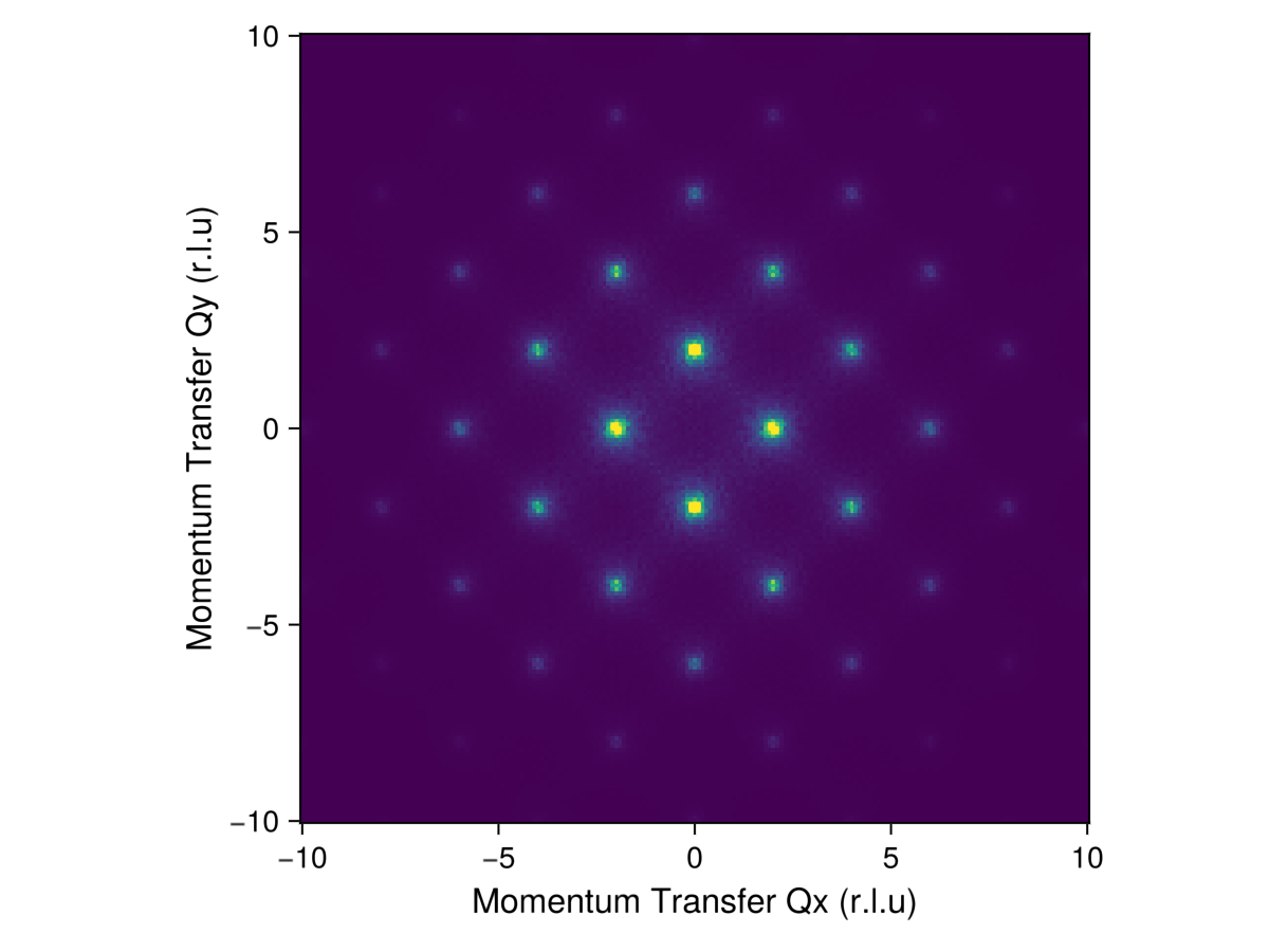
Instantaneous structure factor

To visualize the instantaneous (equal-time) structure factor, create an object instant_correlations. Use add_sample! to accumulate data for each equilibrated spin configuration.

sc = instant_correlations(sys)
add_sample!(sc, sys)    # Accumulate the newly sampled structure factor into `sf`

Collect 20 additional decorrelated samples. For each sample, about 100 Langevin time-steps is sufficient to collect approximately uncorrelated statistics.

for _ in 1:20
    for _ in 1:100
        step!(sys, langevin)
    end
    add_sample!(sc, sys)
end

Define a slice of momentum space. Wavevectors are specified in reciprocal lattice units (RLU). The notation q1s in -10:0.1:10 indicates that the first $q$-component ranges from -10 to 10 in intervals of 0.1. That is, $q$ spans over 20 Brillouin zones. To convert to absolute momentum units, each component of $q$ would need to be scaled by a reciprocal lattice vector.

q1s = -10:0.1:10
q2s = -10:0.1:10
qs = [[q1, q2, 0.0] for q1 in q1s, q2 in q2s];

Plot the instantaneous structure factor for the given $q$-slice. We employ the appropriate FormFactor for Co2⁺. An intensity_formula defines how dynamical correlations correspond to the observable structure factor. The function instant_intensities_interpolated calculates intensities at the target qs by interpolating over the data available at discrete reciprocal-space lattice points.

formfactors = [FormFactor("Co2")]
instant_formula = intensity_formula(sc, :perp; formfactors)
iq = instant_intensities_interpolated(sc, qs, instant_formula);

Plot the resulting intensity data $I(𝐪)$. The color scale is clipped to 50% of the maximum intensity.

heatmap(q1s, q2s, iq;
    colorrange = (0, maximum(iq)/2),
    axis = (
        xlabel="Momentum Transfer Qx (r.l.u)", xlabelsize=16,
        ylabel="Momentum Transfer Qy (r.l.u)", ylabelsize=16,
        aspect=true,
    )
)

Dynamical structure factor

To collect statistics for the dynamical structure factor intensities $I(𝐪,ω)$ at finite temperature, use dynamical_correlations. The integration timestep dt used for measuring dynamical correlations can be somewhat larger than that used by the Langevin dynamics. We must also specify nω and ωmax, which determine the frequencies over which intensity data will be collected.

dt = 2*langevin.dt
ωmax = 6.0  # Maximum energy to resolve (meV)
nω = 50     # Number of energies to resolve
sc = dynamical_correlations(sys; dt, nω, ωmax)

SampledCorrelations (620.429 MiB)
[S(q,ω) | nω = 50, Δω = 0.1259 | 0 sample]
Lattice: (10, 10, 10)×8
6 correlations in Dipole mode:
╔ ⬤ ⬤ ⬤ Sx
║ ⋅ ⬤ ⬤ Sy
╚ ⋅ ⋅ ⬤ Sz

Use Langevin dynamics to sample spin configurations from thermal equilibrium. For each sample, use add_sample! to run a classical spin dynamics trajectory and measure dynamical correlations. Here we average over just 5 samples, but this number could be increased for better statistics.

for _ in 1:5
    for _ in 1:100
        step!(sys, langevin)
    end
    add_sample!(sc, sys)
end

Select points that define a piecewise-linear path through reciprocal space, and a sampling density.

points = [[3/4, 3/4,   0],
          [  0,   0,   0],
          [  0, 1/2, 1/2],
          [1/2,   1,   0],
          [  0,   1,   0],
          [1/4,   1, 1/4],
          [  0,   1,   0],
          [  0,  -4,   0]]
density = 50 # (Å)
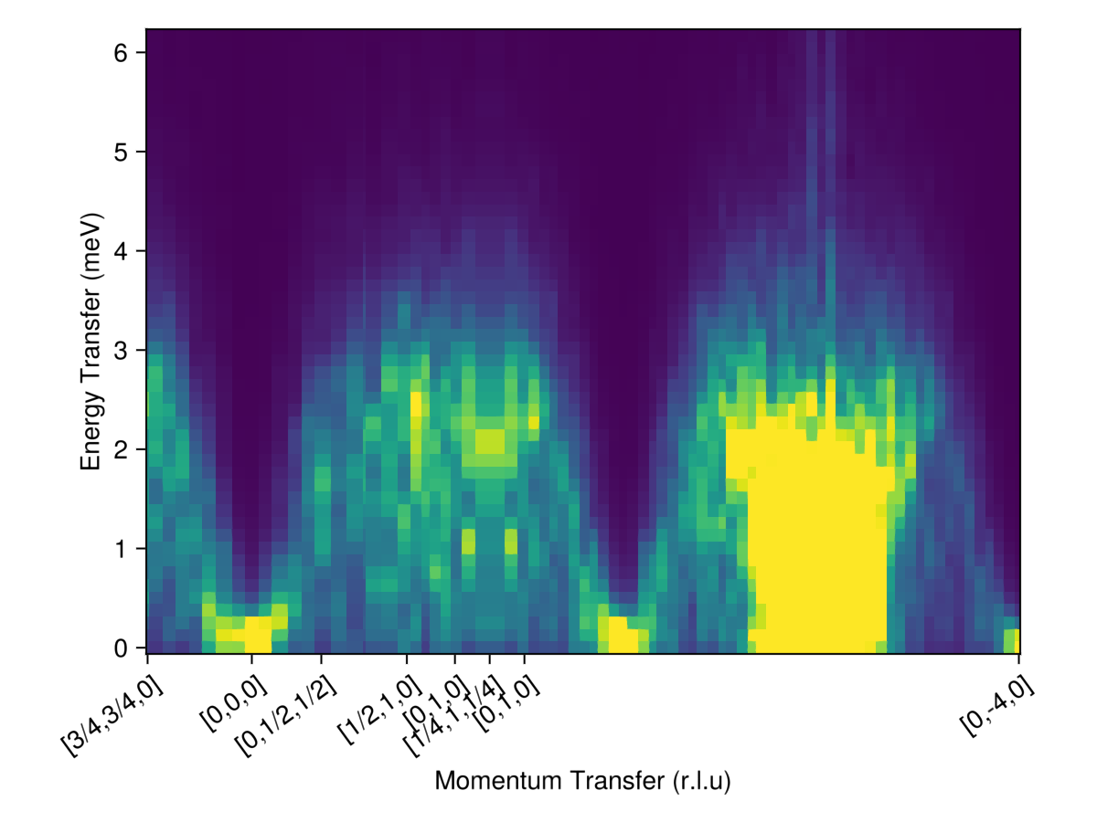
path, xticks = reciprocal_space_path(cryst, points, density);

Calculate $I(𝐪, ω)$ intensities along this path with Lorentzian broadening on the scale of 0.1 meV.

formula = intensity_formula(sc, :perp; formfactors, kT=langevin.kT)
fwhm = 0.2
iqw = intensities_interpolated(sc, path, formula)
iqwc = broaden_energy(sc, iqw, (ω, ω₀) -> lorentzian(; fwhm)(ω-ω₀));

Plot the intensity data on a clipped color scale

ωs = available_energies(sc)
heatmap(1:size(iqwc, 1), ωs, iqwc;
    colorrange = (0, maximum(iqwc)/50),
    axis = (;
        xlabel="Momentum Transfer (r.l.u)",
        ylabel="Energy Transfer (meV)",
        xticks,
        xticklabelrotation=π/5,
        aspect = 1.4,
    )
)

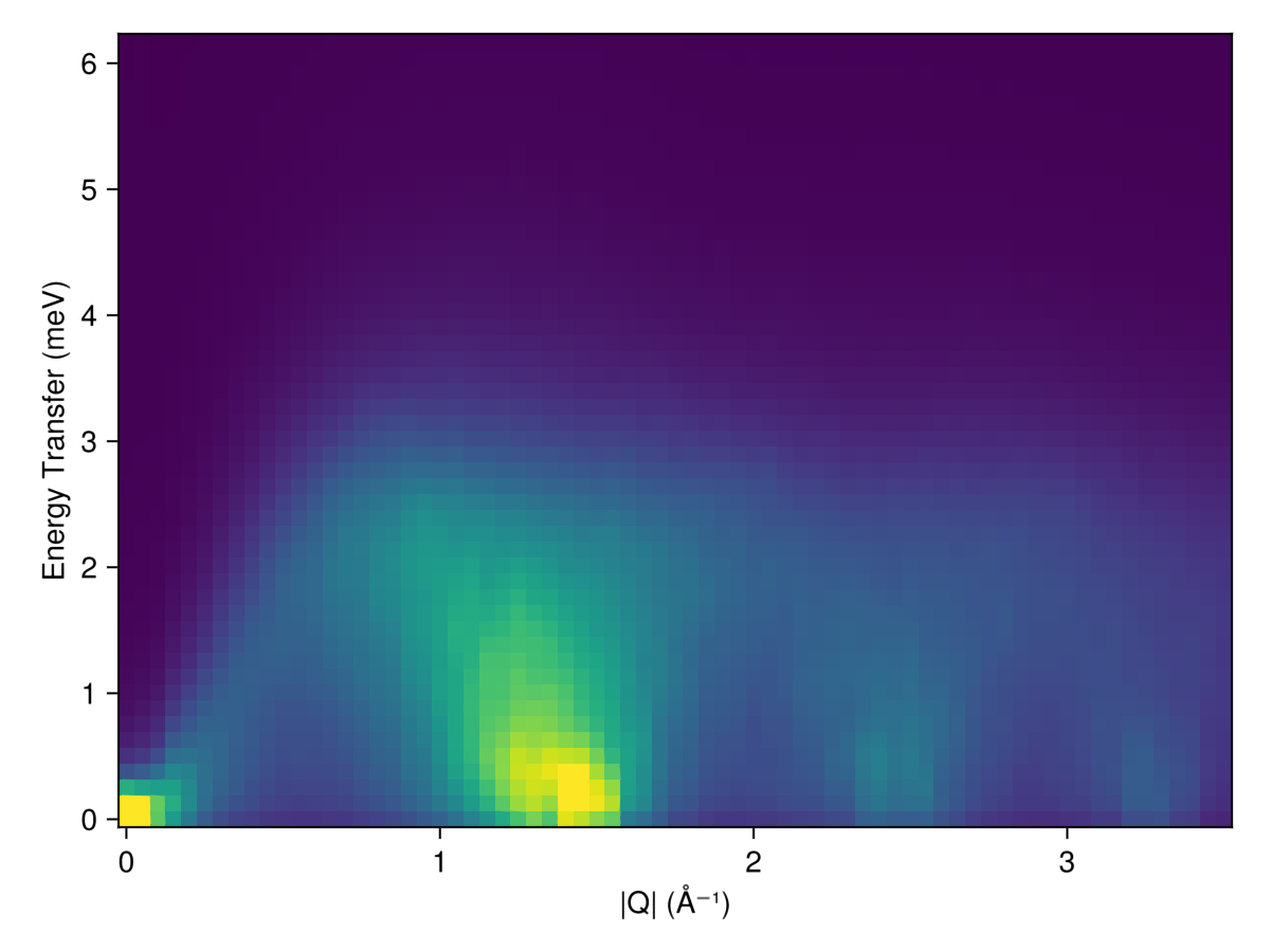
Powder averaged intensity

Define spherical shells in reciprocal space via their radii, in absolute units of 1/Å. For each shell, calculate and average the intensities at 100 $𝐪$-points, sampled approximately uniformly.

radii = 0:0.05:3.5 # (1/Å)
output = zeros(Float64, length(radii), length(ωs))
for (i, radius) in enumerate(radii)
    pts = reciprocal_space_shell(sc.crystal, radius, 100)
    is = intensities_interpolated(sc, pts, formula)
    is = broaden_energy(sc, is, (ω,ω₀) -> lorentzian(; fwhm)(ω-ω₀))
    output[i, :] = mean(is , dims=1)[1,:]
end

Plot resulting powder-averaged structure factor

heatmap(radii, ωs, output;
    axis = (
        xlabel="|Q| (Å⁻¹)",
        ylabel="Energy Transfer (meV)",
        aspect = 1.4,
    ),
    colorrange = (0, 20.0)
)