Download this example as Jupyter notebook or Julia script.

6. Dynamical quench into CP² skyrmion liquid

This example demonstrates Sunny's ability to simulate the out-of-equilibrium dynamics of generalized spin systems. We will implement the model Hamiltonian of Zhang et al., Nature Communications 14, 3626 (2023), which supports a novel type of topological defect, a CP² skyrmion, that involves both the dipolar and quadrupolar parts of a quantum spin.

Beginning from an initial high-temperature state, a disordered gas of CP² skyrmions can be formed by rapidly quenching to low temperature. To model the coupled dynamics of dipoles and quadrupoles, Sunny uses a recently developed generalization of the Landau-Lifshitz spin dynamics, Dahlbom et al., Phys. Rev. B 106, 235154 (2022).

using Sunny, GLMakie

The Hamiltonian we will implement,

\[\mathcal{H} = \sum_{\langle i,j \rangle} J_{ij}( \hat{S}_i^x \hat{S}_j^x + \hat{S}_i^y \hat{S}_j^y + \Delta\hat{S}_i^z \hat{S}_j^z) - h\sum_{i}\hat{S}_i^z + D\sum_{i}(\hat{S}_i^z)^2\]

contains competing ferromagnetic nearest-neightbor and antiferromagnetic next-nearest-neighbor exchange terms on a triangular lattice. Both exchanges exhibit anisotropy on the z-term. Additionally, there is an external magnetic field, $h$, and easy-plane single-ion anisotropy, $D > 0$. We begin by implementing the Crystal.

lat_vecs = lattice_vectors(1, 1, 10, 90, 90, 120)
basis_vecs = [[0,0,0]]
cryst = Crystal(lat_vecs, basis_vecs)

Crystal
Spacegroup 'P 6/m m m' (191)
Lattice params a=1, b=1, c=10, α=90°, β=90°, γ=120°
Cell volume 8.66
Wyckoff 1a (point group '6/mmm'):
   1. [0, 0, 0]

Create a spin System containing $L×L$ cells. Selecting Units.theory with $g=-1$ provides a dimensionless Zeeman coupling of the form $-𝐁⋅𝐬$.

L = 40
dims = (L, L, 1)
sys = System(cryst, dims, [SpinInfo(1, S=1, g=-1)], :SUN; seed=101)

System [SU(3)]
Lattice (40×40×1)×1
Energy per site 0

We proceed to implement each term of the Hamiltonian, selecting our parameters so that the system occupies a region of the phase diagram that supports skyrmions. The exchange interactions are set as follows.

J1 = -1           # Nearest-neighbor ferromagnetic
J2 = (2.0/(1+√5)) # Tune competing exchange to set skyrmion scale length
Δ = 2.6           # Exchange anisotropy

ex1 = J1 * [1 0 0;
            0 1 0;
            0 0 Δ]
ex2 = J2 * [1 0 0;
            0 1 0;
            0 0 Δ]
set_exchange!(sys, ex1, Bond(1, 1, [1, 0, 0]))
set_exchange!(sys, ex2, Bond(1, 1, [1, 2, 0]))

Next we add the external field,

h = 15.5
field = set_field!(sys, [0, 0, h])

and finally an easy-plane single-ion anisotropy,

D = 19.0
set_onsite_coupling!(sys, S -> D*S[3]^2, 1)

Initialize system to an infinite temperature (fully randomized) initial condition.

We will study a temperature quench process using a generalized Langevin spin dynamics. In this SU(3) treatment of quantum spin-1, the dynamics include coupled dipoles and quadrupoles. Select a relatively small damping magnitude to overcome local minima, and disable thermal fluctuations.

damping = 0.05
kT = 0

The first step is to determine a reasonable integration timestep. To determine this, we can initialize the system to some relatively low-energy configuration. A relatively large error tolerance of 0.025 is OK for this phenomenological study.

randomize_spins!(sys)
minimize_energy!(sys) # (this optimization does not need to converge)
integrator = Langevin(; damping, kT)
suggest_timestep(sys, integrator; tol=0.025)

┌ Warning: Optimization failed to converge within 1000 iterations (0.079 ≰ 1e-10)
└ @ Sunny ~/work/Sunny.jl/Sunny.jl/src/Optimization.jl:146
Consider dt ≈ 0.09503 for this spin configuration at tol = 0.025.

Apply the suggested timestep.

integrator.dt = 0.01

0.01

Now run the dynamical quench starting from a randomized configuration. We will record the state of the system at three different times during the quenching process by copying the coherents field of the System.

randomize_spins!(sys)
τs = [4, 16, 256]   # Times to record snapshots
frames = []         # Empty array to store snapshots
for i in eachindex(τs)
    dur = i == 1 ? τs[1] : τs[i] - τs[i-1] # Determine the length of time to simulate
    numsteps = round(Int, dur/integrator.dt)
    for _ in 1:numsteps                    # Perform the integration
        step!(sys, integrator)
    end
    push!(frames, copy(sys.coherents))     # Save a snapshot spin configuration
end

To visualize the state of the system contained in each snapshot, we will calculate and plot the skyrmion density on each plaquette of our lattice. The function plot_triangular_plaquettes is not part of the core Sunny package, but rather something you could define yourself. We are using the definition in plotting2d.jl from the Sunny examples/extra directory.

include(pkgdir(Sunny, "examples", "extra", "Plotting", "plotting2d.jl"))

function sun_berry_curvature(z₁, z₂, z₃)
    z₁, z₂, z₃ = normalize.((z₁, z₂, z₃))
    n₁ = z₁ ⋅ z₂
    n₂ = z₂ ⋅ z₃
    n₃ = z₃ ⋅ z₁
    return angle(n₁ * n₂ * n₃)
end

plot_triangular_plaquettes(sun_berry_curvature, frames; size=(600,200),
    offset_spacing=10, texts=["\tt = "*string(τ) for τ in τs], text_offset=(0, 6)
)

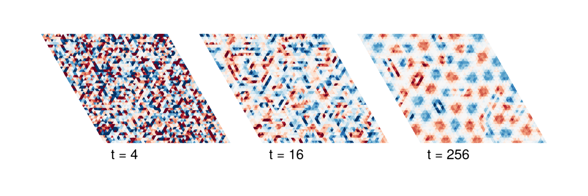
The times are given in $\hbar/|J_1|$. The white background corresponds to a quantum paramagnetic state, where the local spin exhibits a strong quadrupole moment and little or no dipole moment. At late times, there are well-formed skyrmions of positive (red) and negative (blue) charge, and various metastable spin configurations. A full-sized version of this figure is available in Dahlbom et al..