Download this example as Jupyter notebook or Julia script.
7. Long-range dipole interactions
This example demonstrates Sunny's ability to incorporate long-range dipole interactions using Ewald summation. The calculation reproduces previous results in Del Maestro and Gingras, J. Phys.: Cond. Matter, 16, 3339 (2004).
using Sunny, GLMakieCreate a Pyrochlore crystal from spacegroup 227.
latvecs = lattice_vectors(10.19, 10.19, 10.19, 90, 90, 90)
positions = [[0, 0, 0]]
cryst = Crystal(latvecs, positions, 227, setting="2")

units = Units(:meV)
sys = System(cryst, (1, 1, 1), [SpinInfo(1, S=7/2, g=2)], :dipole, seed=2)
J1 = 0.304 * units.K
set_exchange!(sys, J1, Bond(1, 2, [0,0,0]))
Reshape to the primitive cell with four atoms. To facilitate indexing, the function position_to_site accepts positions with respect to the original (cubic) cell.
shape = [1/2 1/2 0; 0 1/2 1/2; 1/2 0 1/2]
sys_prim = reshape_supercell(sys, shape)

set_dipole!(sys_prim, [+1, -1, 0], position_to_site(sys_prim, [0, 0, 0]))
set_dipole!(sys_prim, [-1, +1, 0], position_to_site(sys_prim, [1/4, 1/4, 0]))
set_dipole!(sys_prim, [+1, +1, 0], position_to_site(sys_prim, [1/4, 0, 1/4]))
set_dipole!(sys_prim, [-1, -1, 0], position_to_site(sys_prim, [0, 1/4, 1/4]))

plot_spins(sys_prim; ghost_radius=8, color=[:red, :blue, :yellow, :purple])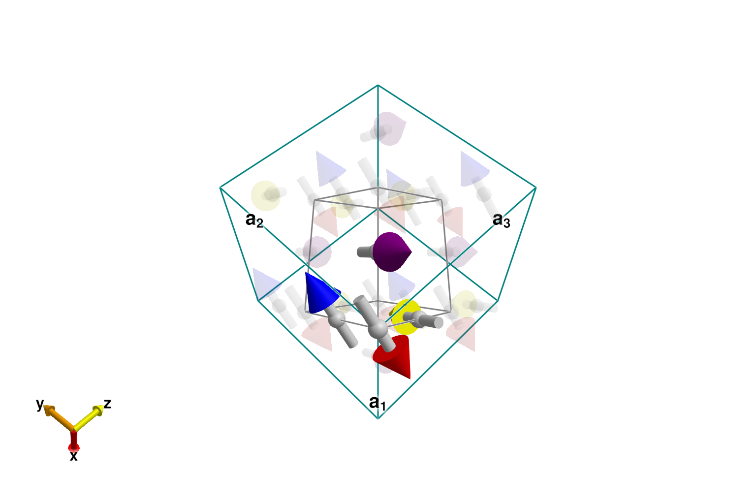
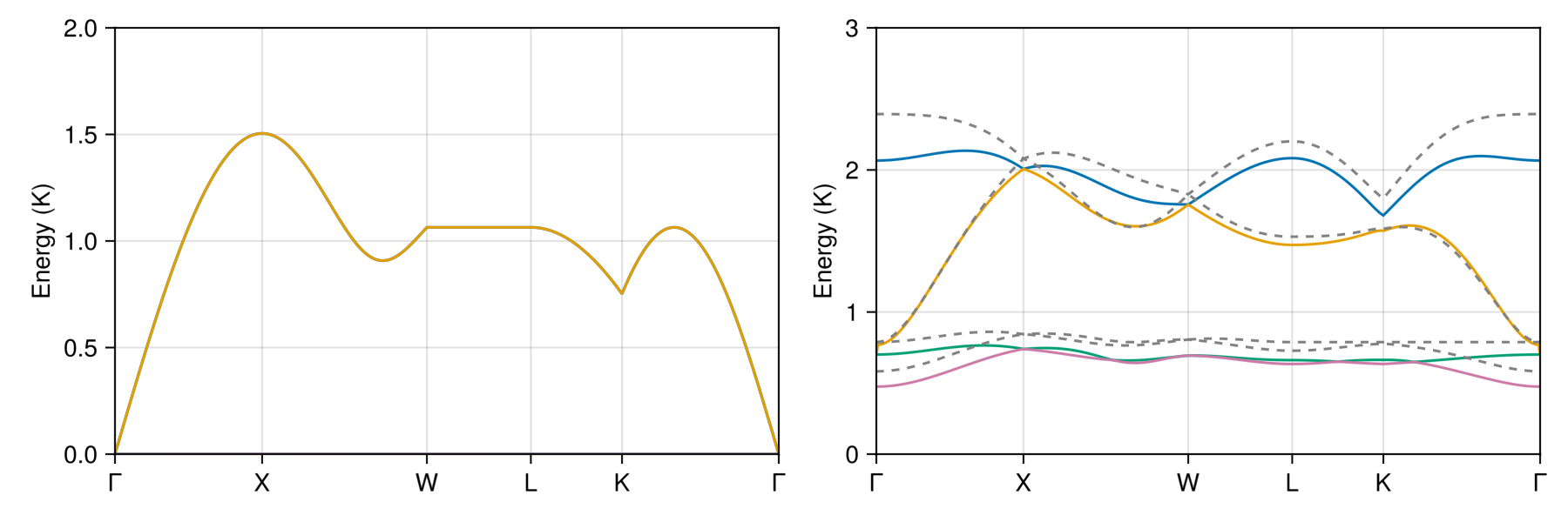
Calculate dispersions with and without long-range dipole interactions. The high-symmetry k-points are specified with respect to the conventional cubic cell.
q_points = [[0,0,0], [0,1,0], [1,1/2,0], [1/2,1/2,1/2], [3/4,3/4,0], [0,0,0]]
q_labels = ["Γ","X","W","L","K","Γ"]
density = 150
path, xticks = reciprocal_space_path(cryst, q_points, density)
xticks = (xticks[1], q_labels)

swt = SpinWaveTheory(sys_prim)
disp1 = dispersion(swt, path)

sys_prim_dd = clone_system(sys_prim)
enable_dipole_dipole!(sys_prim_dd)
swt = SpinWaveTheory(sys_prim_dd)
disp2 = dispersion(swt, path)

sys_prim_tdd = clone_system(sys_prim)
modify_exchange_with_truncated_dipole_dipole!(sys_prim_tdd, 5.0)
swt = SpinWaveTheory(sys_prim_tdd)
disp3 = dispersion(swt, path);
┌ Warning: Deprecated syntax! Consider `enable_dipole_dipole!(sys, units.vacuum_permeability)` where `units = Units(:meV)`.
└ @ Sunny ~/work/Sunny.jl/Sunny.jl/src/System/Interactions.jl:95
┌ Warning: Deprecated syntax! Consider `modify_exchange_with_truncated_dipole_dipole!(sys, cutoff, units.vacuum_permeability)` where `units = Units(:meV)`.
└ @ Sunny ~/work/Sunny.jl/Sunny.jl/src/System/Ewald.jl:264To reproduce Fig. 2 of Del Maestro and Gingras, an empirical rescaling of energy is necessary.
fudge_factor = 1/2 # To reproduce prior work

fig = Figure(size=(900,300))

ax = Axis(fig[1,1]; xlabel="", ylabel="Energy (K)", xticks, xticklabelrotation=0)
ylims!(ax, 0, 2)
xlims!(ax, 1, size(disp1, 1))
for i in axes(disp1, 2)
    lines!(ax, 1:length(disp1[:,i]), fudge_factor*disp1[:,i]/units.K)
end

ax = Axis(fig[1,2]; xlabel="", ylabel="Energy (K)", xticks, xticklabelrotation=0)
ylims!(ax, 0.0, 3)
xlims!(ax, 1, size(disp2, 1))
for i in axes(disp2, 2)
    lines!(ax, 1:length(disp2[:,i]), fudge_factor*disp2[:,i]/units.K)
end

for i in axes(disp3, 2)
    lines!(ax, 1:length(disp3[:,i]), fudge_factor*disp3[:,i]/units.K; color=:gray, linestyle=:dash)
end

fig