Download this example as Jupyter notebook or Julia script.
8. Momentum transfer conventions
This example illustrates Sunny's conventions for dynamical structure factor intensities, $\mathcal{S}(𝐪,ω)$, as documented in the page Structure Factor Calculations. In the neutron scattering context, the variables $𝐪$ and $ω$ describe momentum and energy transfer to the sample.
For systems without inversion-symmetry, the structure factor intensities at $± 𝐪$ may be inequivalent. To highlight this inequivalence, we will construct a 1D chain with Dzyaloshinskii–Moriya interactions between nearest neighbor bonds, and apply a magnetic field.
using Sunny, GLMakieSelecting the P1 spacegroup will effectively disable all symmetry analysis. This can be a convenient way to avoid symmetry-imposed constraints on the couplings. A disadvantage is that all bonds are treated as inequivalent, and Sunny will therefore not be able to propagate any couplings between bonds.
latvecs = lattice_vectors(2, 2, 1, 90, 90, 90)
cryst = Crystal(latvecs, [[0,0,0]], "P1")
Crystal
Spacegroup 'P 1' (1)
Lattice params a=2, b=2, c=1, α=90°, β=90°, γ=90°
Cell volume 4
Class 1:
1. [0, 0, 0]
Construct a 1D chain system that extends along $𝐚₃$. The Hamiltonian includes DM and Zeeman coupling terms, $ℋ = ∑_j D ẑ ⋅ (𝐒_j × 𝐒_{j+1}) - ∑_j 𝐁 ⋅ μ_j$, where $μ_j = - μ_B g 𝐒_j$ is the magnetic_moment and $𝐁 ∝ ẑ$.
sys = System(cryst, (1, 1, 25), [SpinInfo(1; S=1, g=2)], :dipole; seed=0)
D = 0.1 # meV
B = 5D # ~ 8.64T
set_exchange!(sys, dmvec([0, 0, D]), Bond(1, 1, [0, 0, 1]))
set_field!(sys, [0, 0, B])
The large external field fully polarizes the system. Here, the DM coupling contributes nothing, leaving only Zeeman coupling.
randomize_spins!(sys)
minimize_energy!(sys)
@assert energy_per_site(sys) ≈ -10D
Sample from the classical Boltzmann distribution at a low temperature.
dt = 0.1
kT = 0.02
damping = 0.1
langevin = Langevin(dt; kT, damping)
suggest_timestep(sys, langevin; tol=1e-2)
for _ in 1:10_000
    step!(sys, langevin)
end
Consider dt ≈ 0.0995 for this spin configuration at tol = 0.01. Current value is dt = 0.1.The Zeeman coupling polarizes the magnetic moments in the $𝐁 ∝ ẑ$ direction. The spin dipoles, however, are anti-aligned with the magnetic moments, and therefore point towards $-ẑ$. This is shown below.
plot_spins(sys)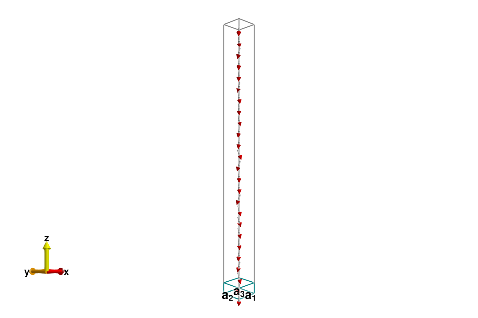
Estimate the dynamical structure factor using classical dynamics.
sc = dynamical_correlations(sys; dt, nω=100, ωmax=15D)
add_sample!(sc, sys)
nsamples = 100
for _ in 1:nsamples
for _ in 1:1_000
step!(sys, langevin)
end
add_sample!(sc, sys)
end
density = 100
path, xticks = reciprocal_space_path(cryst, [[0,0,-1/2], [0,0,+1/2]], density)
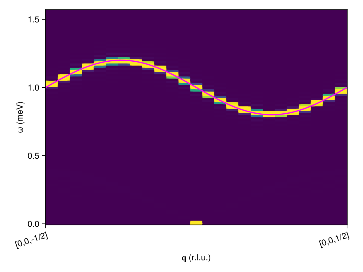
data = intensities_interpolated(sc, path, intensity_formula(sc, :trace; kT));Calculate the same quantity with linear spin wave theory at $T = 0$. Because the ground state is fully polarized, the required magnetic cell is a $1×1×1$ grid of chemical unit cells.
sys_small = resize_supercell(sys, (1,1,1))
minimize_energy!(sys_small)
swt = SpinWaveTheory(sys_small)
formula = intensity_formula(swt, :trace; kernel=delta_function_kernel)
disp_swt, intens_swt = intensities_bands(swt, path, formula);
This model system has a single magnon band with dispersion $ϵ(𝐪) = 1 - 0.2 \sin(2πq₃)$ and uniform intensity. Both calculation methods reproduce this analytical solution. Observe that $𝐪$ and $-𝐪$ are inequivalent. The structure factor calculated from classical dynamics additionally shows an elastic peak at $𝐪 = [0,0,0]$, reflecting the ferromagnetic ground state.
fig = Figure()
ax = Axis(fig[1,1]; aspect=1.4, ylabel="ω (meV)", xlabel="𝐪 (r.l.u.)",
          xticks, xticklabelrotation=π/10)
heatmap!(ax, 1:size(data, 1), available_energies(sc), data;  colorrange=(0.0, 50.0))
lines!(ax, disp_swt[:,1]; color=:magenta, linewidth=2)
fig