Download this example as Jupyter notebook or Julia script.

SW18 - Distorted kagome

This is a Sunny port of SpinW Tutorial 18, originally authored by Goran Nilsen and Sandor Toth. This tutorial illustrates Sunny's experimental for studying incommensurate, single-$Q$ structures. The test system is KCu₃As₂O₇(OD)₃. The Cu ions are arranged in a distorted kagome lattice, and exhibit helical magnetic order, as described in G. J. Nilsen, et al., Phys. Rev. B 89, 140412 (2014).

using Sunny, GLMakie

Build the distorted kagome crystal, with spacegroup 12.

latvecs = lattice_vectors(10.2, 5.94, 7.81, 90, 117.7, 90)
positions = [[0, 0, 0], [1/4, 1/4, 0]]
types = ["Cu1", "Cu2"]
cryst = Crystal(latvecs, positions, 12; types, setting="b1")
view_crystal(cryst)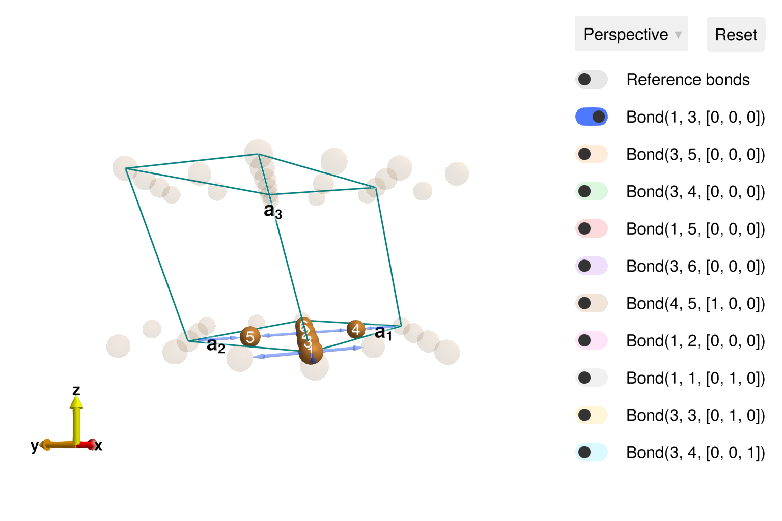

Define the interactions.

spininfos = [SpinInfo(1, S=1/2, g=2), SpinInfo(3, S=1/2, g=2)]
sys = System(cryst, (1,1,1), spininfos, :dipole, seed=0)
J   = -2
Jp  = -1
Jab = 0.75
Ja  = -J/.66 - Jab
Jip = 0.01
set_exchange!(sys, J, Bond(1, 3, [0, 0, 0]))
set_exchange!(sys, Jp, Bond(3, 5, [0, 0, 0]))
set_exchange!(sys, Ja, Bond(3, 4, [0, 0, 0]))
set_exchange!(sys, Jab, Bond(1, 2, [0, 0, 0]))
set_exchange!(sys, Jip, Bond(3, 4, [0, 0, 1]))

Optimize the generalized spiral structure. This will determine the propagation wavevector k, as well as spin values within the unit cell. One must provide a fixed axis perpendicular to the polarization plane. For this system, all interactions are rotationally invariant, and the axis vector is arbitrary. In other cases, a good axis will frequently be determined from symmetry considerations. The qualified notation Sunny.* indicates that these functions are not stabilized, and may change between Sunny releases.

axis = [0, 0, 1]
randomize_spins!(sys)
k = Sunny.minimize_energy_spiral!(sys, axis; k_guess=randn(3))
plot_spins(sys; dims=2)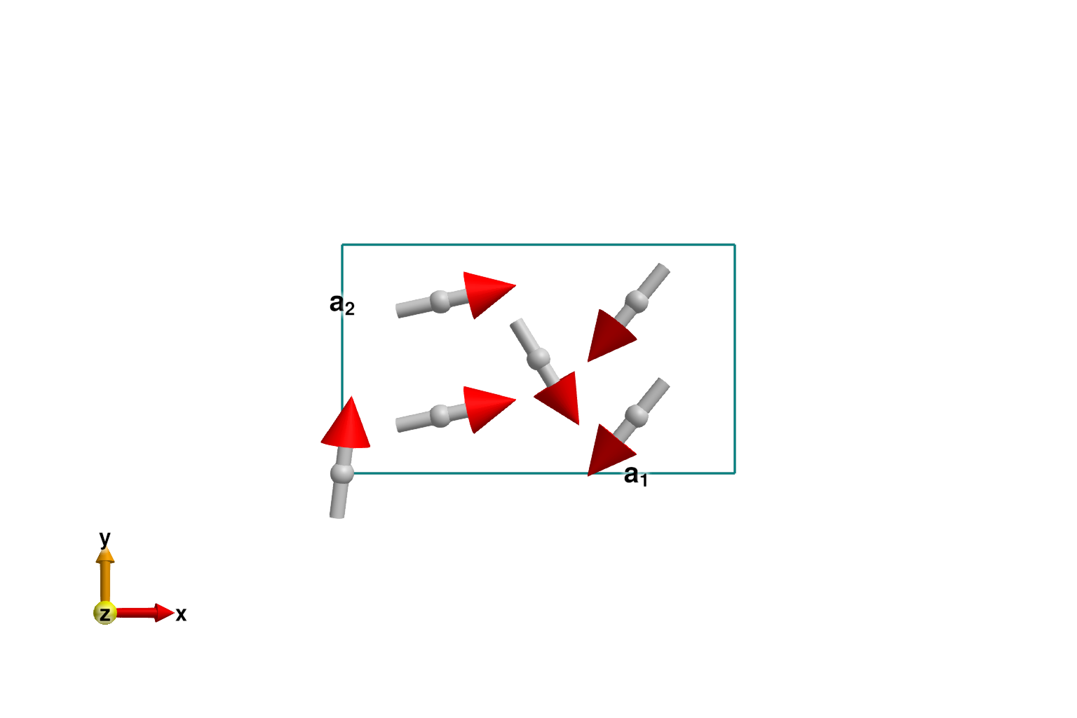

If successful, the optimization process will find one two possible wavevectors, ±k_ref, with opposite chiralities.

k_ref = [0.785902495, 0.0, 0.107048756]
k_ref_alt = [1, 0, 1] - k_ref
@assert isapprox(k, k_ref; atol=1e-6) || isapprox(k, k_ref_alt; atol=1e-6)
@assert Sunny.spiral_energy_per_site(sys; k, axis) ≈ -0.78338383838

Check the energy with a real-space calculation using a large magnetic cell. First, we must determine a lattice size for which k becomes approximately commensurate.

suggest_magnetic_supercell([k_ref]; tol=1e-3)

Possible magnetic supercell in multiples of lattice vectors:

    [14 0 1; 0 1 0; 0 0 2]

for the rationalized wavevectors:

    [[11/14, 0, 3/28]]

Resize the system as suggested, and perform a real-space calculation. Working with a commensurate wavevector increases the energy slightly. The precise value might vary from run-to-run due to trapping in a local energy minimum.

new_shape = [14 0 1; 0 1 0; 0 0 2]
sys2 = reshape_supercell(sys, new_shape)
randomize_spins!(sys2)
minimize_energy!(sys2)
energy_per_site(sys2) # < -0.7834 meV

-0.7791966901275342

Now return to the perfectly incommensurate single-k order. Define a path in reciprocal space.

q_points = [[0,0,0], [1,0,0]]
density = 200
path, xticks = reciprocal_space_path(cryst, q_points, density)
swt = SpinWaveTheory(sys)
formula = Sunny.intensity_formula_spiral(swt, :perp; k, axis, kernel=delta_function_kernel)
disp, _ = intensities_bands(swt, path, formula);
energies = collect(0:0.01:5.5)
broadened_formula = Sunny.intensity_formula_spiral(swt, :perp; k, axis,
                                                   kernel=gaussian(fwhm=0.1))
is = intensities_broadened(swt, path, energies, broadened_formula);

Create the plot

fig = Figure()
ax = Axis(fig[1,1]; xlabel="Momentum (r.l.u.)", ylabel="Energy (meV)",
          title="Spin wave dispersion: ", xticks)
ylims!(ax, 0, 5)
heatmap!(ax, 1:size(is, 1), energies, is; colorrange=(0.2, 100),
         colormap=Reverse(:thermal), lowclip=:white)
for d in eachcol(disp)
    lines!(ax, d; color=:black)
end
fig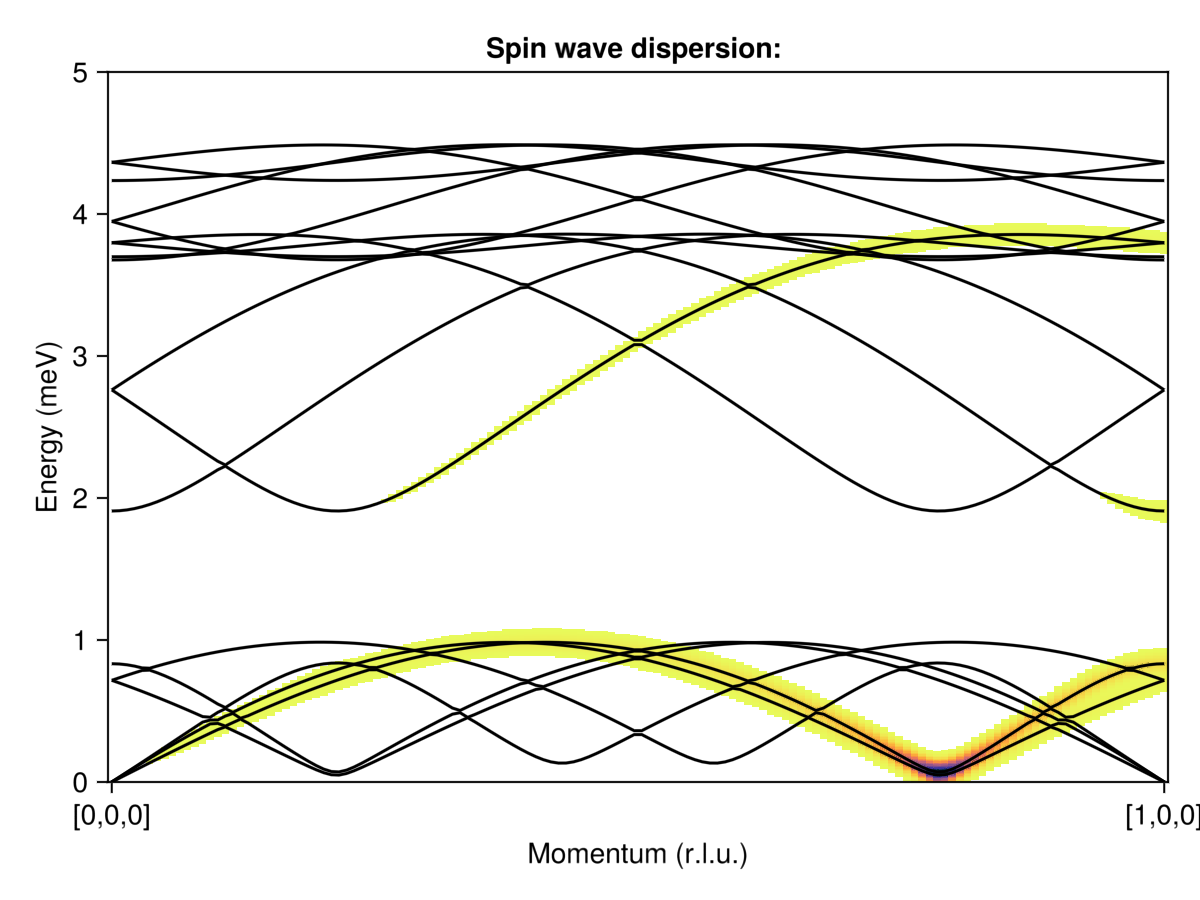

The powder average can be calculated as shown below. It is commented out for now because the calculation is a bit slow to run and is yet to be optimized.

if false
    radii = 0.01:0.02:3
    output = zeros(Float64, length(radii), length(energies))
    for (i, radius) in enumerate(radii)
        n = 300
        qs = reciprocal_space_shell(cryst, radius, n)
        is1 = intensities_broadened(swt, qs, energies, broadened_formula)
        is2 = dropdims(sum(is1[:,:,:,:], dims=[3,4]), dims=(3,4))
        output[i, :] = sum(is2, dims=1) / size(is2, 1)
    end

    fig = Figure()
    ax = Axis(fig[1,1]; xlabel="Q (Å⁻¹)", ylabel="ω (meV)", title="Broadened powder spectra")
    ylims!(ax, 0.0, 5)
    heatmap!(ax, radii, energies, output, colormap=:gnuplot2, colorrange=(0.0,1))
    fig
end