Download this example as Julia file or Jupyter notebook.

1. Spin wave simulations of CoRh₂O₄

This tutorial introduces Sunny through its features for performing conventional spin wave theory calculations. We consider the crystal CoRh₂O₄ and reproduce the calculations of Ge et al., Phys. Rev. B 96, 064413.

Get Julia and Sunny

Sunny is implemented in Julia, which allows for interactive development (like Python or Matlab) while also providing high numerical efficiency (like C++ or Fortran). New Julia users should begin with our Getting Started guide. Sunny requires Julia 1.10 or later.

From the Julia prompt, load Sunny and also GLMakie for graphics.

using Sunny, GLMakie

If these packages are not yet installed, Julia will offer to install them. If executing this tutorial gives an error, you may need to update Sunny and GLMakie from the built-in package manager.

Units

The Units object selects reference energy and length scales, and uses these to provide physical constants. For example, units.K returns one kelvin as 0.086 meV, where the Boltzmann constant is implicit.

units = Units(:meV, :angstrom);

Crystal cell

A crystallographic cell may be loaded from a .cif file, or specified from atom positions and types.

Start by defining the shape of the conventional chemical cell. CoRh₂O₄ has cubic spacegroup 227 (Fd-3m). Its lattice constants are 8.5 Å, and the cell angles are 90°. With this information, lattice_vectors constructs a 3×3 matrix latvecs. Columns of latvecs define the lattice vectors $(𝐚_1, 𝐚_2, 𝐚_3)$ in the global Cartesian coordinate system. Conversely, columns of inv(latvecs) define the global Cartesian axes $(\hat{x}, \hat{y}, \hat{z})$ in components of the lattice vectors.

a = 8.5031 # (Å)
latvecs = lattice_vectors(a, a, a, 90, 90, 90)

3×3 StaticArraysCore.SMatrix{3, 3, Float64, 9} with indices SOneTo(3)×SOneTo(3):
 8.5031  0.0     0.0
 0.0     8.5031  0.0
 0.0     0.0     8.5031

Construct the Crystal cell from the spacegroup number 227 and one representative atom of each occupied Wyckoff. In the standard setting of spacegroup 227, position [0, 0, 0] belongs to Wyckoff 8a, which is the diamond cubic crystal.

positions = [[0, 0, 0]]
cryst = Crystal(latvecs, positions, 227; types=["Co"], setting="1")

Crystal
Spacegroup 'F d -3 m' (227)
Lattice params a=8.503, b=8.503, c=8.503, α=90°, β=90°, γ=90°
Cell volume 614.8
Type 'Co', Wyckoff 8a (point group '-43m'):
   1. [0, 0, 0]
   2. [1/2, 1/2, 0]
   3. [1/4, 1/4, 1/4]
   4. [3/4, 3/4, 1/4]
   5. [1/2, 0, 1/2]
   6. [0, 1/2, 1/2]
   7. [3/4, 1/4, 3/4]
   8. [1/4, 3/4, 3/4]

view_crystal launches an interface for interactive inspection and symmetry analysis.

view_crystal(cryst)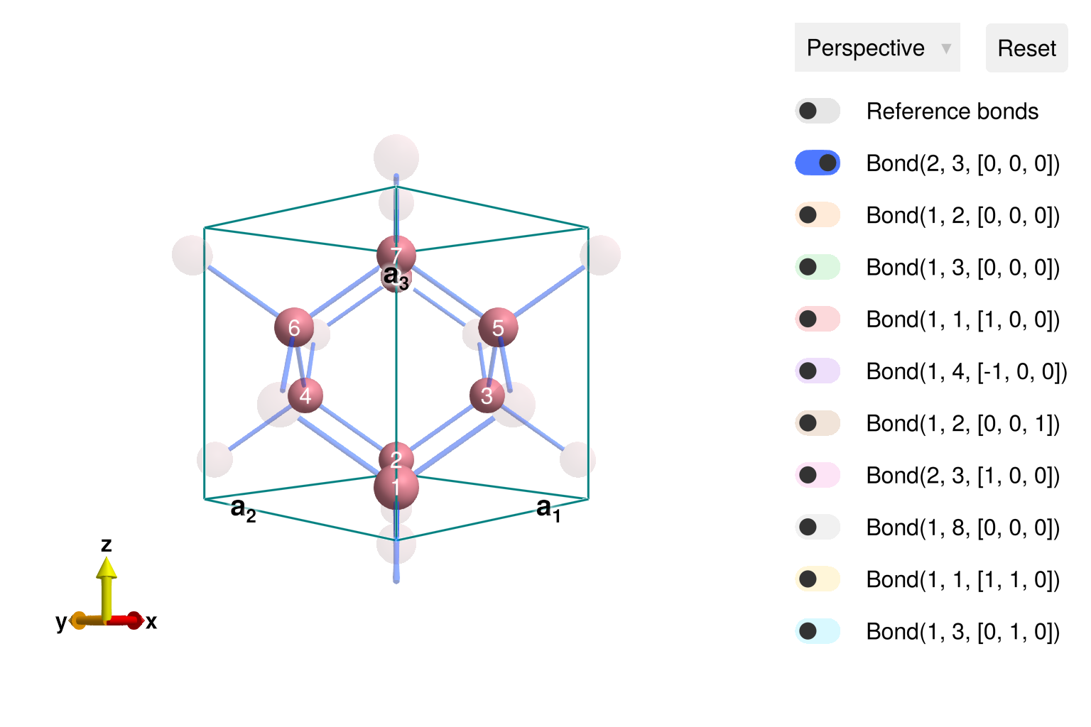

Spin system

A System will define the spin model. Each cobalt atom carries quantum spin $s = 3/2$, with a $g$-factor of 2. Specify this Moment data for cobalt atom 1. By symmetry, the same moment data also applies to cobalt atoms 2, 3, ... 7. The option :dipole indicates a traditional model type, for which quantum spin is modeled as a dipole expectation value.

sys = System(cryst, [1 => Moment(s=3/2, g=2)], :dipole)

System [Dipole mode]
Supercell (1×1×1)×8
Energy per site 0

Ge et al. demonstrated that inelastic neutron scattering data for CoRh₂O₄ is well modeled by antiferromagnetic nearest neighbor exchange, J = 0.63 meV. Call set_exchange! with the bond that connects atom 1 to atom 3, and has zero displacement between chemical cells. Consistent with the symmetries of spacegroup 227, this interaction will be propagated to all other nearest-neighbor bonds. Calling view_crystal with sys now shows the antiferromagnetic Heisenberg interactions as blue polkadot spheres.

J = +0.63 # (meV)
set_exchange!(sys, J, Bond(1, 3, [0, 0, 0]))
view_crystal(sys)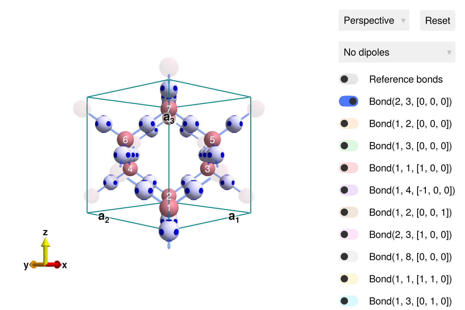

Optimizing spins

To search for the ground state, call randomize_spins! and minimize_energy! in sequence. For this problem, optimization converges rapidly to the expected Néel order. See this with plot_spins, where spins are colored according to their global $z$-component.

randomize_spins!(sys)
minimize_energy!(sys)
plot_spins(sys; color=[S[3] for S in sys.dipoles])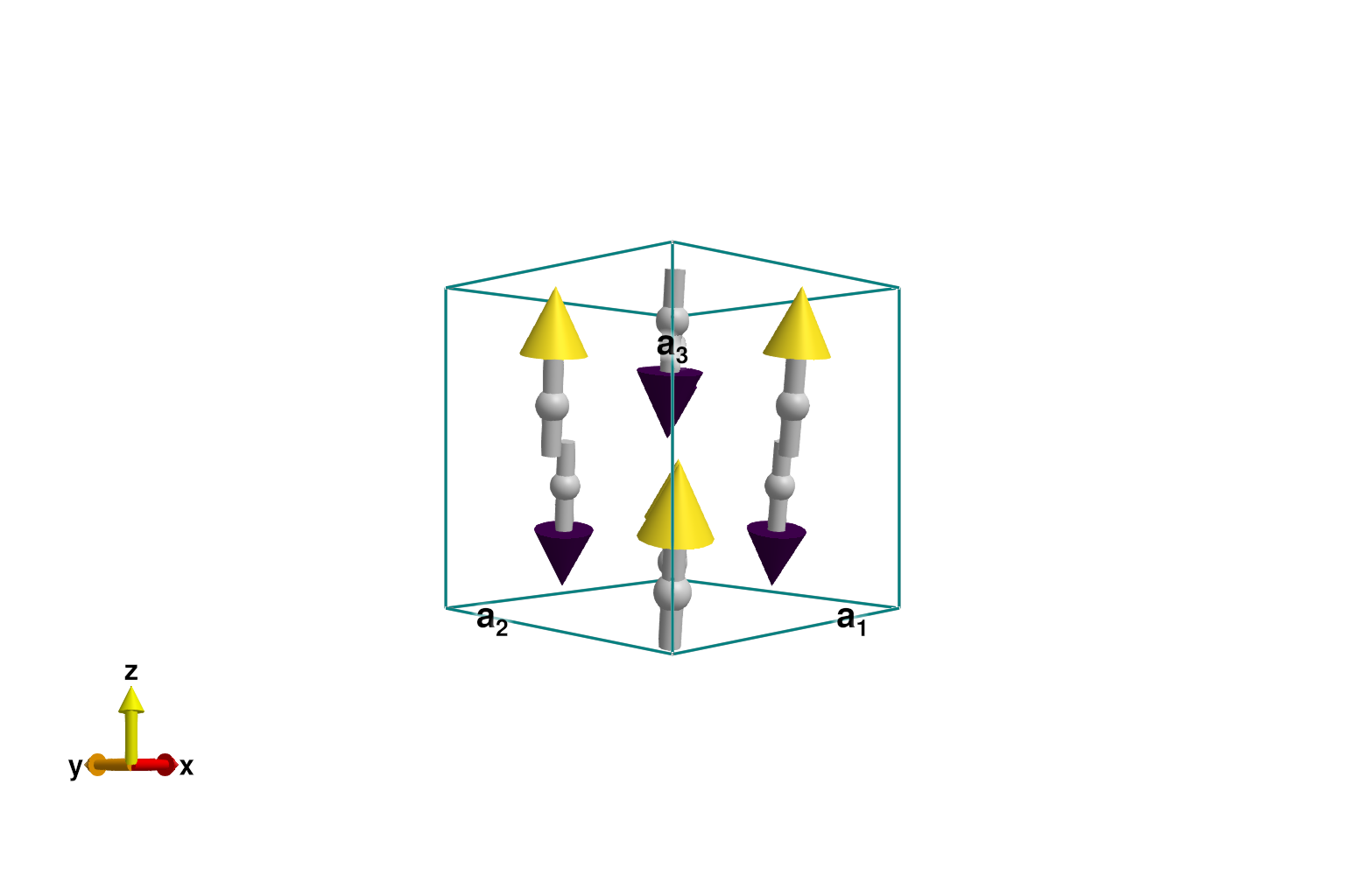

The diamond lattice is bipartite, allowing each spin to perfectly anti-align with its 4 nearest-neighbors. Each of these 4 bonds contribute $-J s^2$ to the total energy. Two sites participate in each bond, so the energy per site is $-2 J s^2$. Check this by calling energy_per_site.

@assert energy_per_site(sys) ≈ -2J*(3/2)^2

Reshaping the magnetic cell

The most compact magnetic cell for this Néel order is a primitive unit cell. Reduce the magnetic cell size using reshape_supercell, where columns of the shape matrix are primitive lattice vectors as multiples of the conventional cubic lattice vectors $(𝐚_1, 𝐚_2, 𝐚_3)$. One could alternatively use shape = cryst.latvecs \ cryst.prim_latvecs. Verify that the energy per site is unchanged after the reshaping the supercell.

shape = [0 1 1;
         1 0 1;
         1 1 0] / 2
sys_prim = reshape_supercell(sys, shape)
@assert energy_per_site(sys_prim) ≈ -2J*(3/2)^2

Plotting sys_prim shows the two spins within the primitive cell, as well as the larger conventional cubic cell for context.

plot_spins(sys_prim; color=[S[3] for S in sys_prim.dipoles])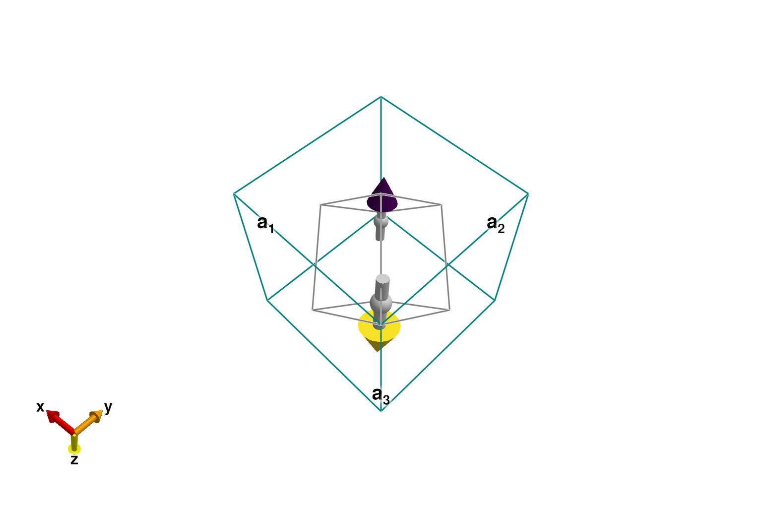

Spin wave theory

With this primitive cell, we will perform a SpinWaveTheory calculation of the structure factor $\mathcal{S}(𝐪,ω)$. The measurement ssf_perp indicates projection of the spin structure factor $\mathcal{S}(𝐪,ω)$ perpendicular to the direction of momentum transfer, as appropriate for unpolarized neutron scattering. The isotropic FormFactor for Co²⁺ dampens intensities at large $𝐪$.

formfactors = [1 => FormFactor("Co2")]
measure = ssf_perp(sys_prim; formfactors)
swt = SpinWaveTheory(sys_prim; measure)

SpinWaveTheory [Dipole mode]
  2 atoms

Select lorentzian broadening with a full-width at half-maximum (FWHM) of 0.8 meV.

kernel = lorentzian(fwhm=0.8)

Broadening

Define a q_space_path that connects high-symmetry points in reciprocal space. The $𝐪$-points are given in reciprocal lattice units (RLU) for the original cubic cell. For example, [1/2, 1/2, 0] denotes the sum of the first two reciprocal lattice vectors, $𝐛_1/2 + 𝐛_2/2$. A total of 500 $𝐪$-points will be sampled along the path.

qs = [[0, 0, 0], [1/2, 0, 0], [1/2, 1/2, 0], [0, 0, 0]]
path = q_space_path(cryst, qs, 500)

QPath (500 samples)
  [0, 0, 0] → [1/2, 0, 0] → [1/2, 1/2, 0] → [0, 0, 0]

Calculate single-crystal scattering intensities along this path, for energies between 0 and 6 meV. Use plot_intensities to visualize the result.

energies = range(0, 6, 300)
res = intensities(swt, path; energies, kernel)
plot_intensities(res; units, title="CoRh₂O₄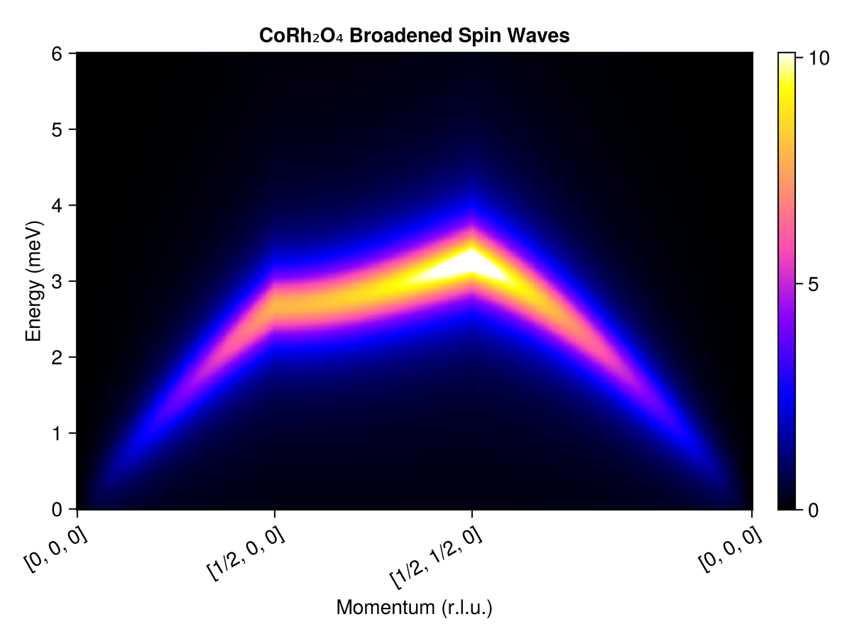 LSWT")

Sometimes experimental data is only available as a powder average, i.e., as an average over all possible crystal orientations. Use powder_average to simulate these intensities. Each $𝐪$-magnitude defines a spherical shell in reciprocal space. Consider 200 radii from 0 to 3 inverse angstroms, and collect 2000 random samples per spherical shell. As configured, this calculation completes in about two seconds. Had we used the conventional cubic cell, the calculation would be an order of magnitude slower.

radii = range(0, 3, 200) # (1/Å)
res = powder_average(cryst, radii, 2000) do qs
    intensities(swt, qs; energies, kernel)
end
plot_intensities(res; units, saturation=1.0, title="CoRh₂O₄ Powder Average")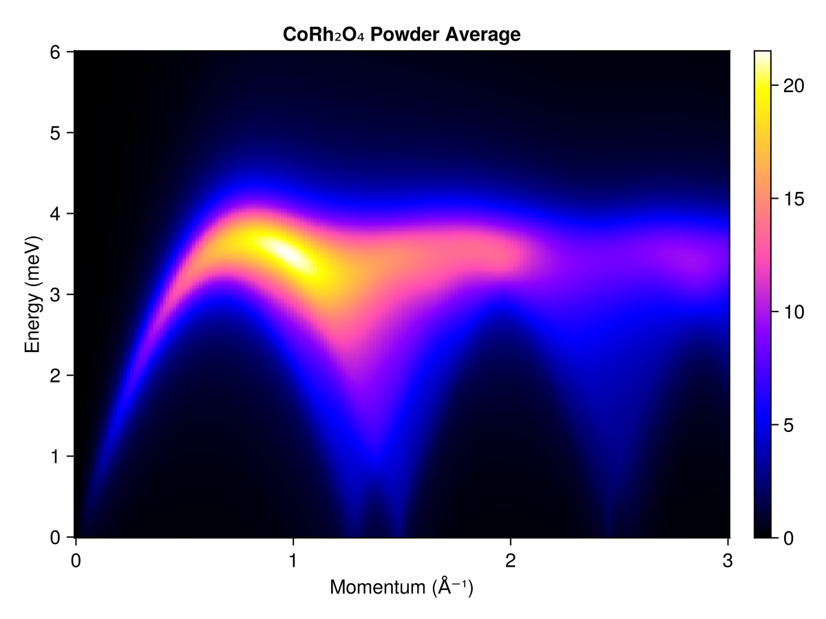

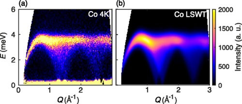
This result can be compared to experimental neutron scattering data from Fig. 5 of Ge et al.

What's next?

For more spin wave calculations of this type, browse the SpinW tutorials ported to Sunny.
Spin wave theory neglects thermal fluctuations of the magnetic order. The next CoRh₂O₄ tutorial demonstrates how to sample spins in thermal equilibrium, and measure dynamical correlations from the classical spin dynamics.
Sunny also offers features that go beyond the dipole approximation of a quantum spin via the theory of SU(N) coherent states. This can be especially useful for systems with strong single-ion anisotropy, as demonstrated in the FeI₂ tutorial.