Download this example as Julia file or Jupyter notebook.

7. Long-range dipole interactions

This example demonstrates long-range dipole-dipole interactions in the context of a spin wave calculation. These interactions can be included two ways: with infinite-range Ewald summation or with a real-space distance cutoff. The study follows Del Maestro and Gingras, J. Phys.: Cond. Matter, 16, 3339 (2004).

using Sunny, GLMakie

Create a pyrochlore crystal from Wyckoff 16c for spacegroup 227.

units = Units(:K, :angstrom)
latvecs = lattice_vectors(10.19, 10.19, 10.19, 90, 90, 90)
positions = [[0, 0, 0]]
cryst = Crystal(latvecs, positions, 227)
view_crystal(cryst)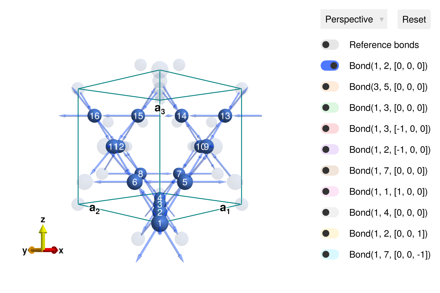

Create a System with a random number seed that was empirically selected to produce the desired type of spontaneous symmetry breaking. Reshape to the primitive cell, which contains four atoms. Add antiferromagnetic nearest neighbor exchange interactions.

sys = System(cryst, [1 => Moment(s=7/2, g=2)], :dipole; seed=0)
sys = reshape_supercell(sys, primitive_cell(cryst))
J1 = 0.304 # (K)
set_exchange!(sys, J1, Bond(1, 2, [0,0,0]))

Create a copy of the system and enable long-range dipole-dipole interactions using Ewald summation.

sys_lr = clone_system(sys)
enable_dipole_dipole!(sys_lr, units.vacuum_permeability)

Create a copy of the system and add long-range dipole-dipole interactions up to a 5 Å cutoff distance.

sys_lr_cut = clone_system(sys)
modify_exchange_with_truncated_dipole_dipole!(sys_lr_cut, 5.0, units.vacuum_permeability)

Find an energy minimizing spin configuration accounting for the long-range dipole-dipole interactions. This will arbitrarily select from a discrete set of possible ground states based on the system seed.

randomize_spins!(sys_lr)
minimize_energy!(sys_lr)
plot_spins(sys_lr; ghost_radius=8, color=[:red, :blue, :yellow, :purple])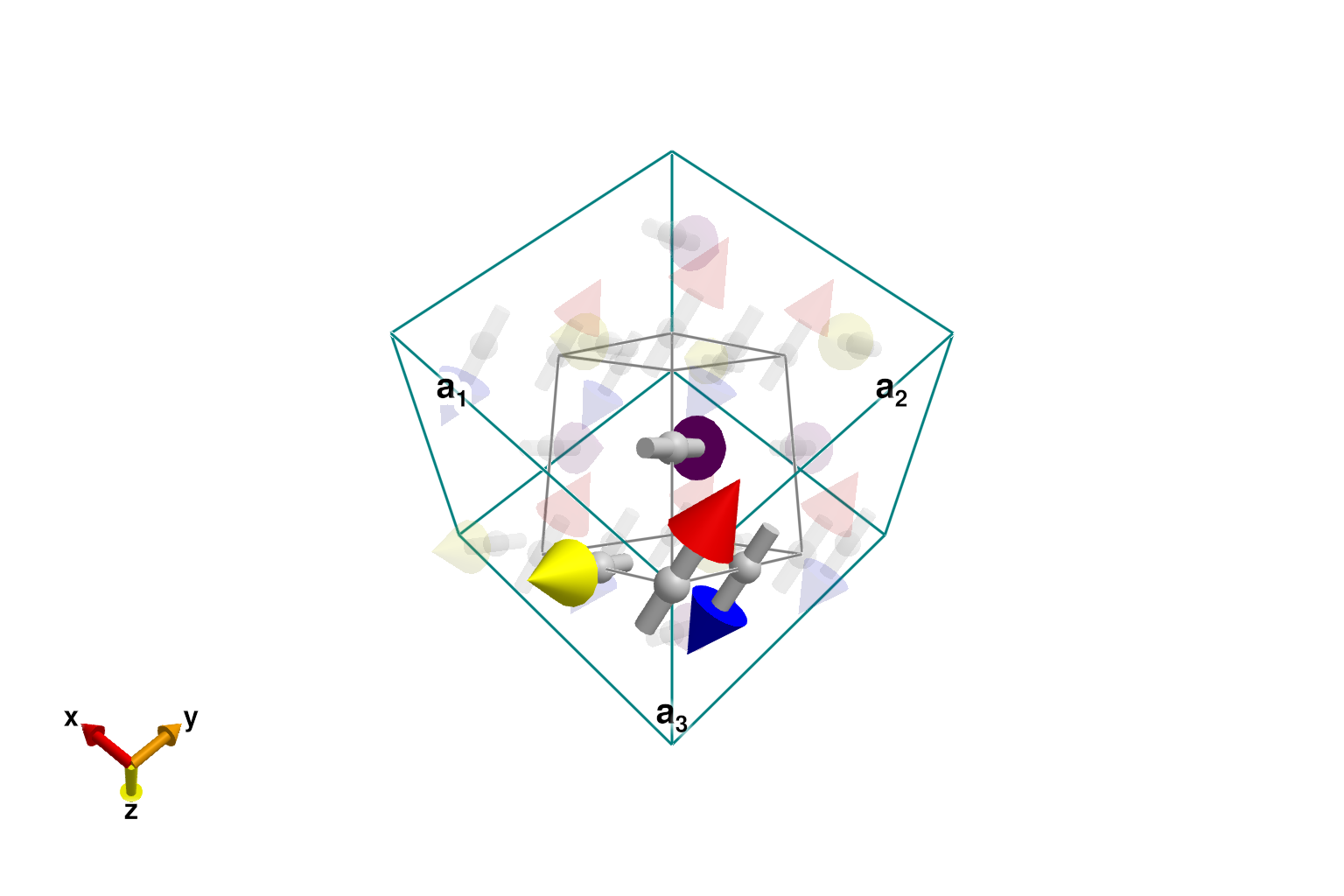

Copy this configuration to the other two systems. Note that the original sys has a continuum of degenerate ground states.

sys.dipoles .= sys_lr.dipoles
sys_lr_cut.dipoles .= sys_lr.dipoles;

Calculate dispersions for the three systems. The high-symmetry $𝐪$-points are specified in reciprocal lattice units with respect to the conventional cubic cell.

qs = [[0,0,0], [0,1,0], [1,1/2,0], [1/2,1/2,1/2], [3/4,3/4,0], [0,0,0]]
labels = ["Γ", "X", "W", "L", "K", "Γ"]
path = q_space_path(cryst, qs, 500; labels)

measure = ssf_trace(sys)
swt = SpinWaveTheory(sys; measure)
res1 = intensities_bands(swt, path)

swt = SpinWaveTheory(sys_lr; measure)
res2 = intensities_bands(swt, path)

swt = SpinWaveTheory(sys_lr_cut; measure)
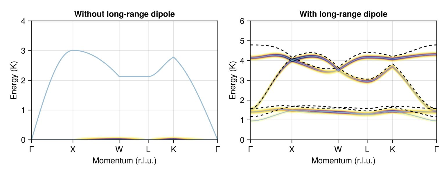
res3 = intensities_bands(swt, path);

Create a panel corresponding to Fig. 2 of Del Maestro and Gingras. Dashed lines show the effect of truncating dipole-dipole interactions at 5 Å. The Del Maestro and Gingras paper underreported the energy scale by a factor of two, and requires slight corrections to its third dispersion band.

fig = Figure(size=(768, 300))
plot_intensities!(fig[1, 1], res1; units, title="Without long-range dipole")
ax = plot_intensities!(fig[1, 2], res2; units, title="With long-range dipole")
for c in eachrow(res3.disp)
    lines!(ax, eachindex(c), c; linestyle=:dash, color=:black)
end
fig