Download this example as Julia file or Jupyter notebook.

4. Generalized spin dynamics of FeI₂ at finite T

The previous FeI₂ tutorial used multi-flavor spin wave theory to calculate the dynamical spin structure factor. This tutorial performs an analogous calculation at finite temperature using the classical dynamics of SU(N) coherent states.

Compared to spin wave theory, classical spin dynamics in real-space is typically much slower, and is limited in $𝐪$-space resolution. The approach, however, allows for thermal fluctuations, can be used to explore finite temperature phases, and enables the study of highly non-equilibrium processes.

The structure of this tutorial largely follows the previous study of CoRh₂O₄ at finite T. The main difference is that CoRh₂O₄ can be well described with :dipole mode, whereas FeI₂ is best modeled using :SUN mode, owing to its strong easy-axis anisotropy.

Construct the FeI₂ system as previously described.

using Sunny, GLMakie

units = Units(:meV, :angstrom)
a = b = 4.05012
c = 6.75214
latvecs = lattice_vectors(a, b, c, 90, 90, 120)
cryst = Crystal(latvecs, [[0,0,0]], 164; types=["Fe"])

sys = System(cryst, [1 => Moment(s=1, g=2)], :SUN)
J1pm   = -0.236
J1pmpm = -0.161
J1zpm  = -0.261
J2pm   = 0.026
J3pm   = 0.166
J′0pm  = 0.037
J′1pm  = 0.013
J′2apm = 0.068
J1zz   = -0.236
J2zz   = 0.113
J3zz   = 0.211
J′0zz  = -0.036
J′1zz  = 0.051
J′2azz = 0.073
J1xx = J1pm + J1pmpm
J1yy = J1pm - J1pmpm
J1yz = J1zpm
set_exchange!(sys, [J1xx 0.0 0.0; 0.0 J1yy J1yz; 0.0 J1yz J1zz], Bond(1,1,[1,0,0]))
set_exchange!(sys, [J2pm 0.0 0.0; 0.0 J2pm 0.0; 0.0 0.0 J2zz], Bond(1,1,[1,2,0]))
set_exchange!(sys, [J3pm 0.0 0.0; 0.0 J3pm 0.0; 0.0 0.0 J3zz], Bond(1,1,[2,0,0]))
set_exchange!(sys, [J′0pm 0.0 0.0; 0.0 J′0pm 0.0; 0.0 0.0 J′0zz], Bond(1,1,[0,0,1]))
set_exchange!(sys, [J′1pm 0.0 0.0; 0.0 J′1pm 0.0; 0.0 0.0 J′1zz], Bond(1,1,[1,0,1]))
set_exchange!(sys, [J′2apm 0.0 0.0; 0.0 J′2apm 0.0; 0.0 0.0 J′2azz], Bond(1,1,[1,2,1]))
D = 2.165
set_onsite_coupling!(sys, S -> -D*S[3]^2, 1)

Thermalization

To study thermal fluctuations in real-space, use a large system size with 16×16×4 copies of the chemical cell.

sys = resize_supercell(sys, (16, 16, 4))

System [SU(3)]
Supercell (16×16×4)×1
Energy per site -353/250

Direct optimization via minimize_energy! is susceptible to trapping in a local minimum. An alternative approach is to simulate the system using Langevin spin dynamics. This requires a bit more set-up, but allows sampling from thermal equilibrium at any target temperature. Select the temperature 2.3 K ≈ 0.2 meV. This temperature is small enough to magnetically order, but large enough so that the dynamics can readily overcome local energy barriers and annihilate defects.

langevin = Langevin(; damping=0.2, kT=2.3*units.K)

Langevin(<missing>; damping=0.2, kT=0.19819866502933906)

Use suggest_timestep to select an integration timestep for the error tolerance tol=1e-2. Initializing sys to some low-energy configuration usually works well.

randomize_spins!(sys)
minimize_energy!(sys; maxiters=10)
suggest_timestep(sys, langevin; tol=1e-2)
langevin.dt = 0.03;

Consider dt ≈ 0.03042 for this spin configuration at tol = 0.01.

Run a Langevin trajectory for 10,000 time-steps and plot the spins. The magnetic order is present, but may be difficult to see.

for _ in 1:10_000
    step!(sys, langevin)
end
plot_spins(sys; color=[S[3] for S in sys.dipoles])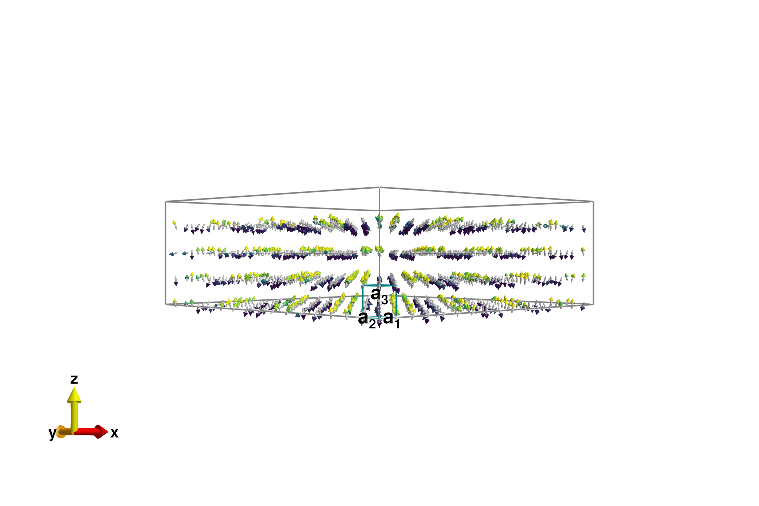

Verify the expected two-up, two-down spiral magnetic order by calling print_wrapped_intensities. A single propagation wavevector $±𝐤$ dominates the static intensity in $\mathcal{S}(𝐪)$, indicating the expected 2 up, 2 down magnetic spiral order. A smaller amount of intensity is spread among many other wavevectors due to thermal fluctuations.

print_wrapped_intensities(sys)

Dominant wavevectors for spin sublattices:

    [-1/4, 1/4, 1/4]       14.01% weight
    [1/4, -1/4, -1/4]      14.01%
    [1/4, 0, 1/4]           7.60%
    [-1/4, 0, -1/4]         7.60%
    [1/4, -0.0625, 1/4]     4.35%
    [-1/4, 0.0625, -1/4]    4.35%
    [-1/4, 0.1875, 1/4]     3.28%
    [1/4, -0.1875, -1/4]    3.28%
    [-1/4, 0.3125, 1/4]     3.00%
    [1/4, -0.3125, -1/4]    3.00%
    [1/4, 0.0625, 1/4]      2.72%
    ...                     ...

Thermalization has not substantially altered the suggested dt.

suggest_timestep(sys, langevin; tol=1e-2)

Consider dt ≈ 0.03267 for this spin configuration at tol = 0.01. Current value is dt = 0.03.

Structure factor in the paramagnetic phase

The remainder of this tutorial will focus on the paramagnetic phase. Re-thermalize the system to the temperature of 3.5 K ≈ 0.30 meV.

langevin.kT = 3.5 * units.K
for _ in 1:10_000
    step!(sys, langevin)
end

The suggested timestep has increased slightly. Following this suggestion will make the simulations a bit faster.

suggest_timestep(sys, langevin; tol=1e-2)
langevin.dt = 0.040;

Consider dt ≈ 0.03972 for this spin configuration at tol = 0.01. Current value is dt = 0.03.

Collect dynamical spin structure factor data using SampledCorrelations. This procedure involves sampling spin configurations from thermal equilibrium and using the spin dynamics of SU(N) coherent states to estimate dynamical correlations. With proper classical-to-quantum corrections, the associated structure factor intensities $S^{αβ}(q,ω)$ can be compared with finite-temperature inelastic neutron scattering data. Incorporate the FormFactor appropriate to Fe²⁺.

dt = 2*langevin.dt
energies = range(0, 7.5, 120)
formfactors = [1 => FormFactor("Fe2"; g_lande=3/2)]
sc = SampledCorrelations(sys; dt, energies, measure=ssf_perp(sys; formfactors))

SampledCorrelations (37.950 MiB)
[S(q,ω) | nω = 119, Δω = 0.063 | 0 sample]
Lattice: (3,) × 1

The function add_sample! will collect data by running a dynamical trajectory starting from the current system configuration.

add_sample!(sc, sys)

To collect additional data, it is required to re-sample the spin configuration from the thermal distribution. Statistical error is reduced by fully decorrelating the spin configurations between calls to add_sample!.

for _ in 1:2
    for _ in 1:1000               # Enough steps to decorrelate spins
        step!(sys, langevin)
    end
    add_sample!(sc, sys)
end

Perform an intensity calculation for two special $𝐪$-points in reciprocal lattice units (RLU). A classical-to-quantum rescaling of normal mode occupations will be performed according to the temperature kT. The large statistical noise could be reduced by averaging over more thermal samples.

res = intensities(sc, [[0, 0, 0], [0.5, 0.5, 0.5]]; energies, langevin.kT)
fig = lines(res.energies, res.data[:, 1]; axis=(xlabel="meV", ylabel="Intensity"), label="(0,0,0)")
lines!(res.energies, res.data[:, 2]; label="(π,π,π)")
axislegend()
fig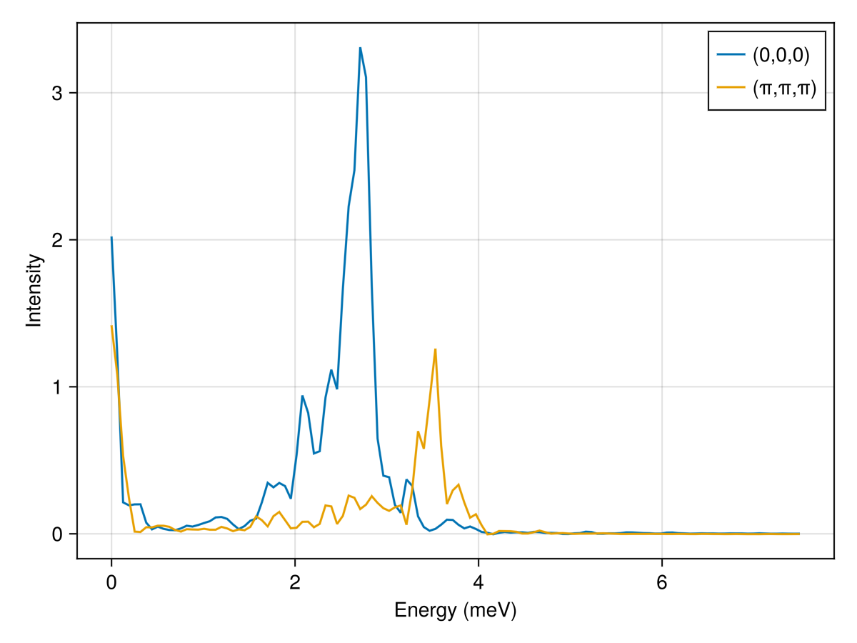

Next, we will measure intensities along a q_space_path that connects high symmetry points. Because this is a real-space calculation, data is only available for discrete $𝐪$ modes, with resolution that scales inversely to linear system size. Intensities at $ω = 0$ dominate, so to enhance visibility, we restrict the color range empirically.

qs = [[0,   0, 0],  # List of wave vectors that define a path
      [1,   0, 0],
      [0,   1, 0],
      [1/2, 0, 0],
      [0,   1, 0],
      [0,   0, 0]]
qpath = q_space_path(cryst, qs, 500)
res = intensities(sc, qpath; energies, langevin.kT)
plot_intensities(res; colorrange=(0.0, 1.0), title="Intensities at T = 2.3 K")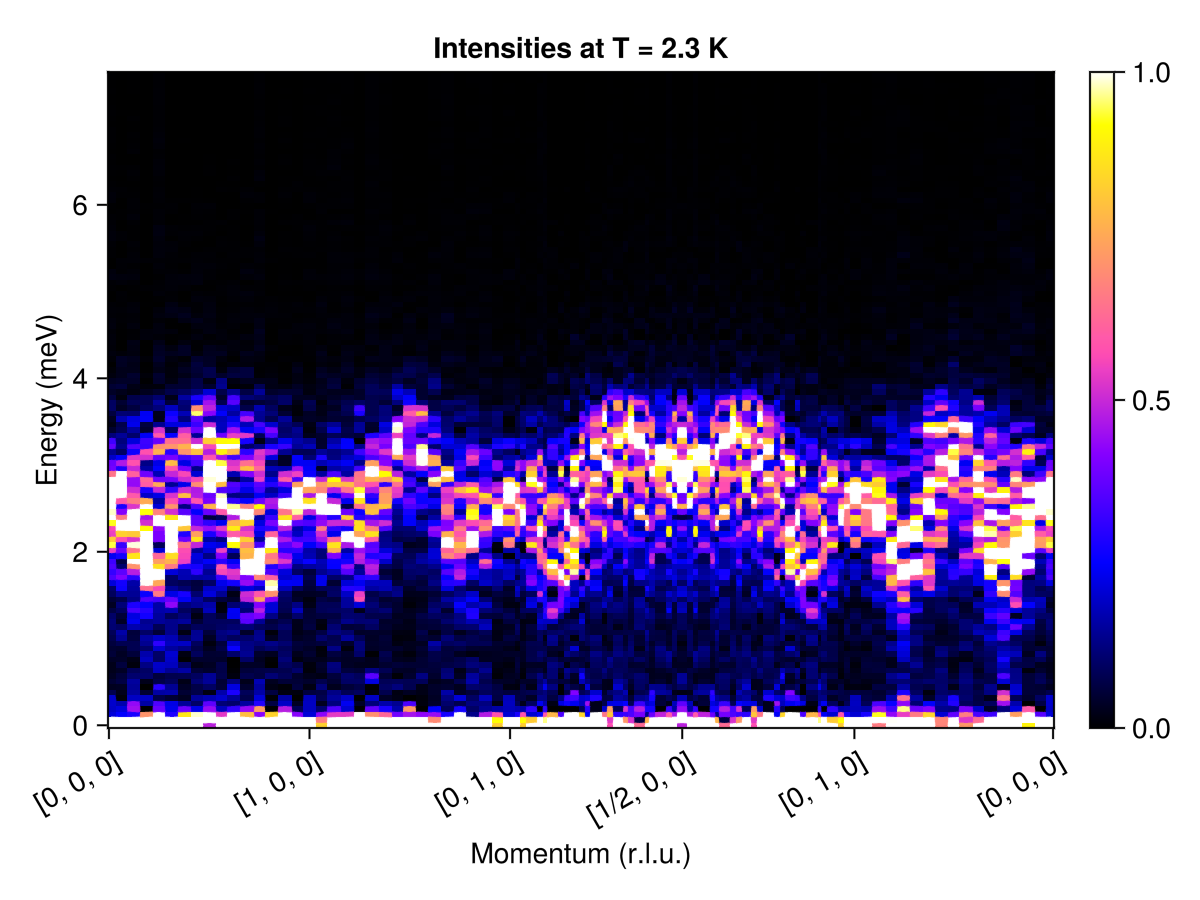

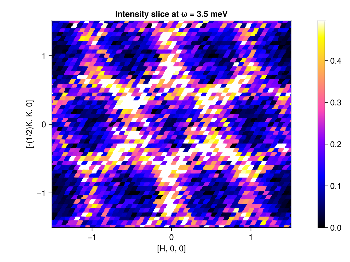
One can also view the intensity along a q_space_grid for a fixed energy value. Alternatively, use intensities_static to integrate over all available energies.

grid = q_space_grid(cryst, [1, 0, 0], range(-1.5, 1.5, 300), [0, 1, 0], (-1.5, 1.5); orthogonalize=true)
res = intensities(sc, grid; energies=[3.5], langevin.kT)
plot_intensities(res; title="Intensity slice at ω = 3.5 meV")