Download this example as Julia file or Jupyter notebook.

SW02 - AFM Heisenberg chain

This is a Sunny port of SpinW Tutorial 2, originally authored by Bjorn Fak and Sandor Toth. It calculates the spin wave spectrum of the antiferromagnetic Heisenberg nearest-neighbor spin chain.

Load Sunny and the GLMakie plotting package

using Sunny, GLMakie

Define the chemical cell for a 1D chain following the previous tutorial.

units = Units(:meV, :angstrom)
latvecs = lattice_vectors(3, 8, 8, 90, 90, 90)
cryst = Crystal(latvecs, [[0, 0, 0]])
view_crystal(cryst; ndims=2, ghost_radius=8)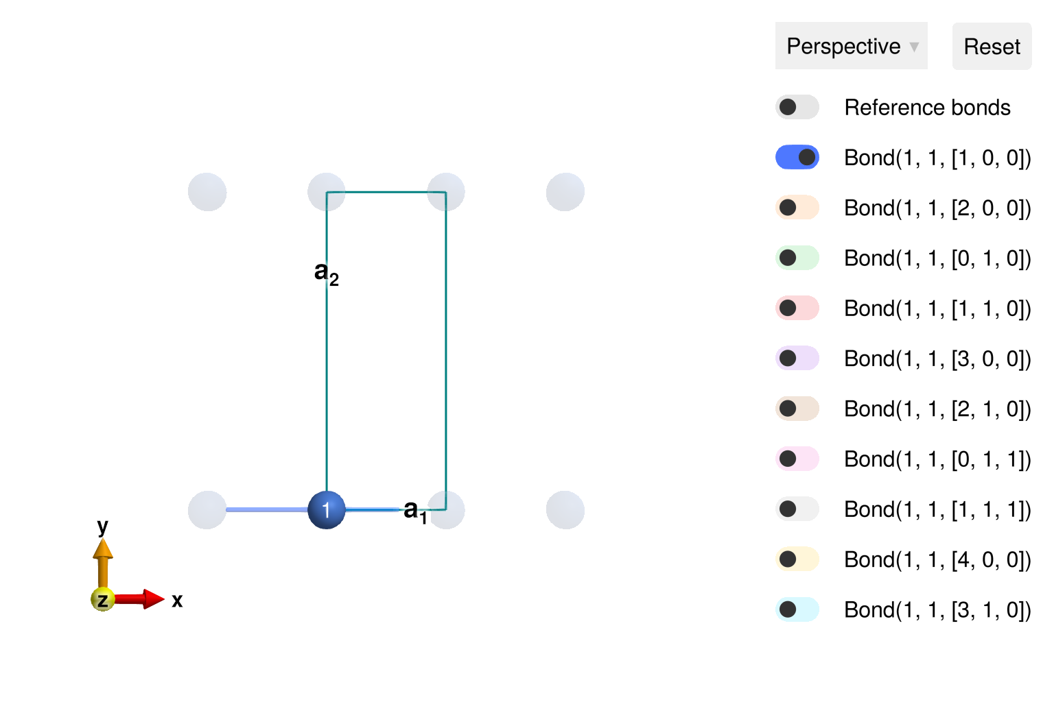

Unlike in the previous tutorial, here the magnetic cell should include 2×1×1 chemical cells to support antiferromagnetic (Néel) order along the chain.

sys = System(cryst, [1 => Moment(s=1, g=2)], :dipole; dims=(2, 1, 1))

System [Dipole mode]
Supercell (2×1×1)×1
Energy per site 0

Set a nearest neighbor interaction of $J = +1$ meV along the chain, and find the energy-minimizing Néel order. As before, a global rotation in spin-space is arbitrary.

J = 1
set_exchange!(sys, J, Bond(1, 1, [1, 0, 0]))
randomize_spins!(sys)
minimize_energy!(sys)
plot_spins(sys; ndims=2, ghost_radius=8)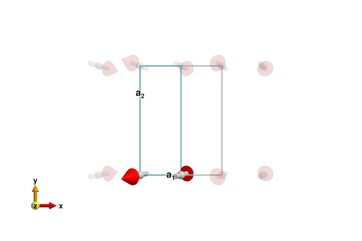

Perform a SpinWaveTheory calculation for a path between $[0,0,0]$ and $[1,0,0]$ in RLU.

swt = SpinWaveTheory(sys; measure=ssf_perp(sys))
qs = [[0,0,0], [1,0,0]]
path = q_space_path(cryst, qs, 400)
res = intensities_bands(swt, path)
plot_intensities(res; units)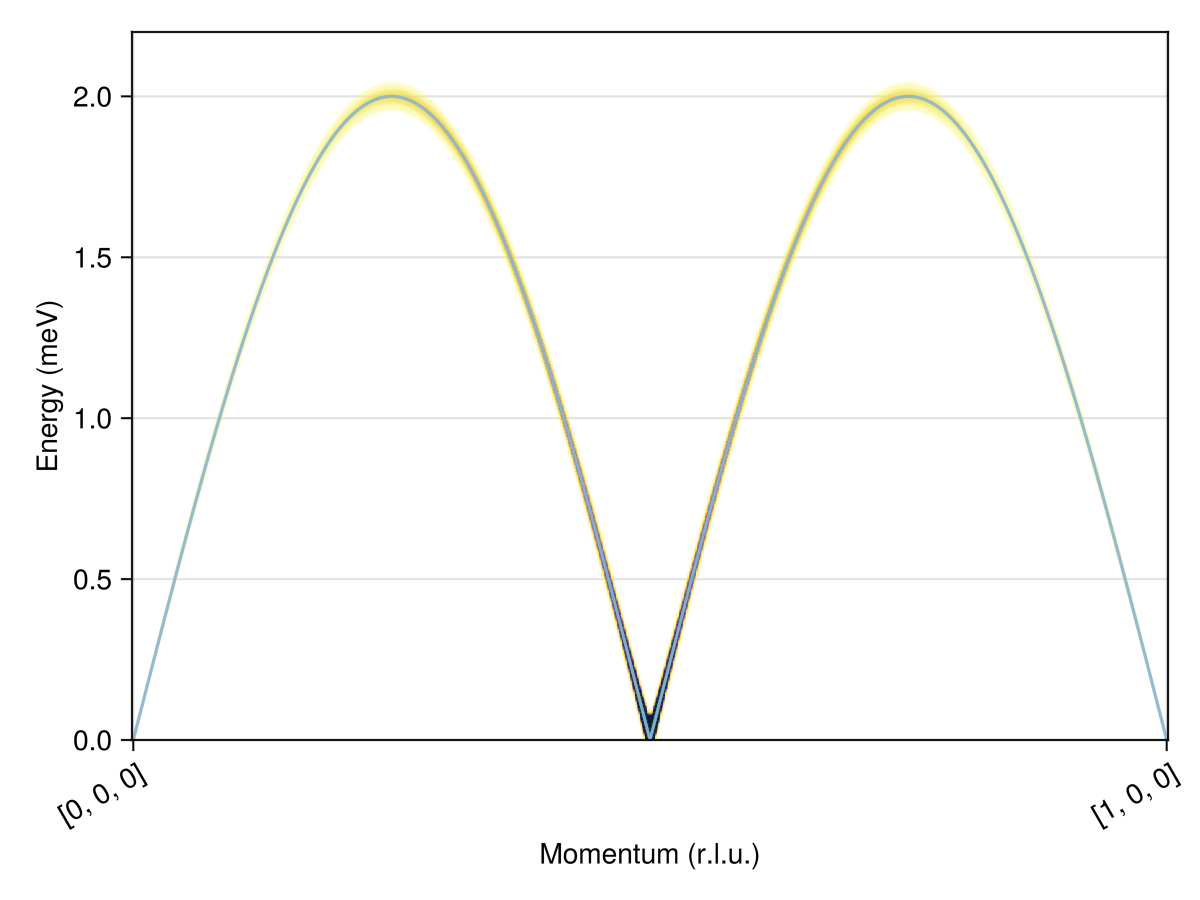

This system includes two bands that are fully degenerate in their dispersion.

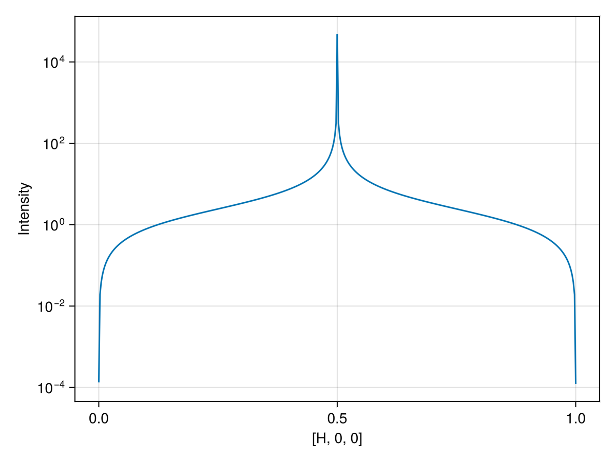
isapprox(res.disp[1, :], res.disp[2, :])

true

Plot the intensities summed over the two degenerate bands using the Makie lines function.

xs = [q[1] for q in path.qs]
ys = log10.(res.data[1, :] + res.data[2, :])
lines(xs, ys; axis=(; xlabel="[H, 0, 0]", ylabel="Log intensity (dimensionless)"))