Download this example as Julia file or Jupyter notebook.
SW05 - Simple kagome ferromagnet
This is a Sunny port of SpinW Tutorial 5, originally authored by Bjorn Fak and Sandor Toth. It calculates the spin wave spectrum of the kagome lattice with a nearest-neighbor ferromagnetic coupling.
Load Sunny and the GLMakie plotting package.
using Sunny, GLMakieDefine the chemical cell. By specifying spacegroup 147 (P-3), Sunny will propagate the position [1/2, 0, 0] to the three symmetry-equivalent sites of the kagome unit cell.
units = Units(:meV, :angstrom)
latvecs = lattice_vectors(6, 6, 5, 90, 90, 120)
positions = [[1/2, 0, 0]]
cryst = Crystal(latvecs, positions, 147)
Crystal
Spacegroup 'P -3' (147)
Lattice params a=6, b=6, c=5, α=90°, β=90°, γ=120°
Cell volume 155.9
Wyckoff 3e (site sym. '-1'):
1. [1/2, 0, 0]
2. [0, 1/2, 0]
3. [1/2, 1/2, 0]
Another way to construct the kagome lattice is to provide all three site positions of the chemical cell and allow Sunny to infer the largest possible group of symmetry operations. In this case, Sunny infers spacegroup 191 (P6/mmm). Because 191 has more symmetry operations than 147, it will impose more constraints on the allowed 3×3 exchange matrices. Isotropic Heisenberg exchange, however, is always allowed.
positions = [[1/2, 0, 0], [0, 1/2, 0], [1/2, 1/2, 0]]
cryst2 = Crystal(latvecs, positions)
Crystal
Spacegroup 'P 6/m m m' (191)
Lattice params a=6, b=6, c=5, α=90°, β=90°, γ=120°
Cell volume 155.9
Wyckoff 3f (site sym. 'mmm'):
1. [1/2, 0, 0]
2. [0, 1/2, 0]
3. [1/2, 1/2, 0]
View the kagome lattice
view_crystal(cryst; ndims=2)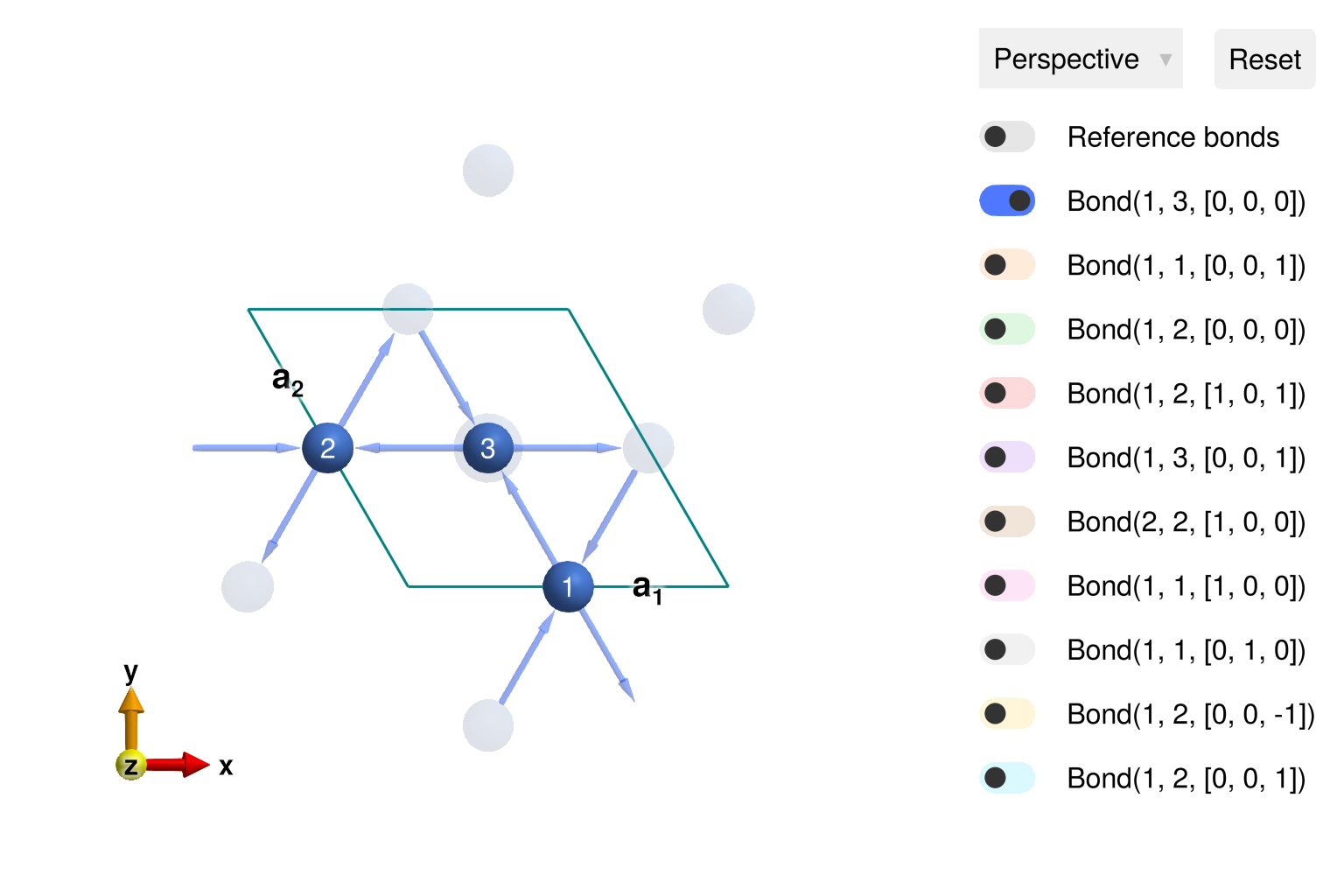
Construct a spin system with nearest-neighbor ferromagnetic interactions.
sys = System(cryst, [1 => Moment(s=1, g=2)], :dipole)
J = -1.0
set_exchange!(sys, J, Bond(2, 3, [0, 0, 0]))
Energy minimization yields the expected ferromagnetic order. Each site participates in 4 bonds, which contributes energy 4J/2.
randomize_spins!(sys)
minimize_energy!(sys)
energy_per_site(sys)
@assert energy_per_site(sys) ≈ 4J/2
plot_spins(sys; ndims=2)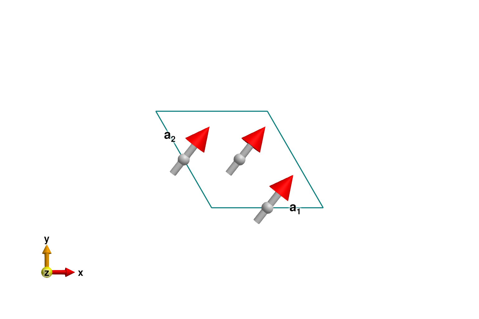
Calculate and plot intensities for a path through $𝐪$-space.
swt = SpinWaveTheory(sys; measure=ssf_perp(sys))
qs = [[-1/2, 0, 0], [0, 0, 0], [1/2, 1/2, 0]]
path = q_space_path(cryst, qs, 400)
res = intensities_bands(swt, path)
plot_intensities(res; units)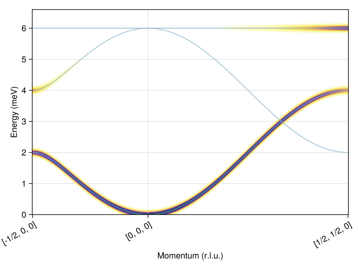
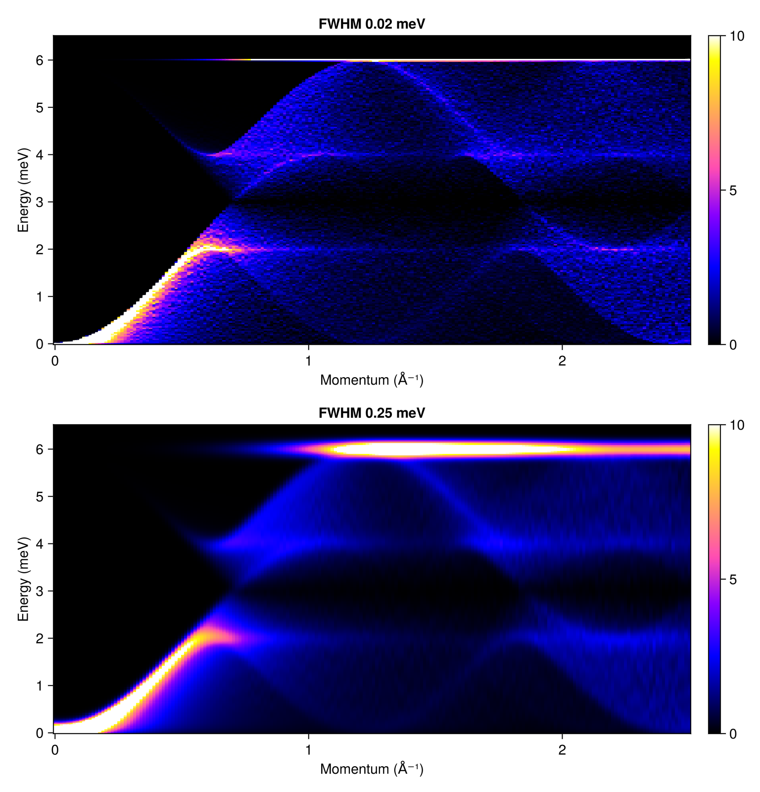
Calculate and plot the powder average with two different magnitudes of Gaussian line-broadening. Pick an explicit intensity colorrange (as a density in meV) so that the two color scales are consistent.
radii = range(0, 2.5, 200)
energies = range(0, 6.5, 200)
res1 = powder_average(cryst, radii, 1000) do qs
    intensities(swt, qs; energies, kernel=gaussian(fwhm=0.02))
end
res2 = powder_average(cryst, radii, 1000) do qs
    intensities(swt, qs; energies, kernel=gaussian(fwhm=0.25))
end

fig = Figure(size=(768, 800))
plot_intensities!(fig[1, 1], res1; units, colorrange=(0,10), title="FWHM 0.02 meV")
plot_intensities!(fig[2, 1], res2; units, colorrange=(0,10), title="FWHM 0.25 meV")
fig