Download this example as Julia file or Jupyter notebook.

SW10 - Energy cut on square lattice

This is a Sunny port of SpinW Tutorial 10, originally authored by Sandor Toth. It calculates the spin wave spectrum on a constant energy cut of the frustrated square lattice.

Load Sunny and the GLMakie plotting package

using Sunny, GLMakie

Define the chemical cell for the 2D square lattice.

units = Units(:meV, :angstrom)
latvecs = lattice_vectors(1.0, 1.0, 3.0, 90, 90, 90)
cryst = Crystal(latvecs, [[0, 0, 0]])

Crystal
Spacegroup 'P 4/m m m' (123)
Lattice params a=1, b=1, c=3, α=90°, β=90°, γ=90°
Cell volume 3
Wyckoff 1a (point group '4/mmm'):
   1. [0, 0, 0]

Construct a spin system with nearest-neighbor antiferomagnetic interactions of 1.0 meV. Energy minimization yields the expected Néel order on the 2×2 magnetic cell.

sys = System(cryst, [1 => Moment(s=1, g=2)], :dipole; dims=(2, 2, 1))
set_exchange!(sys, 1.0, Bond(1, 1, [1, 0, 0]))
randomize_spins!(sys)
minimize_energy!(sys)
plot_spins(sys; ndims=2)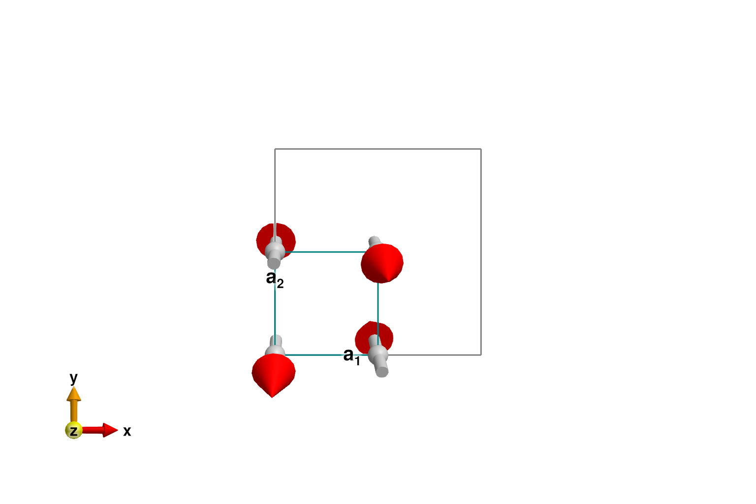

Define a 2D slice through $𝐪$-space with q_space_grid.

grid = q_space_grid(cryst, [1, 0, 0], range(0, 2, 201), [0, 1, 0], range(0, 2, 201))

Sunny.QGrid{2} (201×201 samples)

Calculate and plot a constant energy cut at the precise value of 3.75 meV. Apply a line broadening with a full-width half-max of 0.2 meV to approximately capture intensities between 3.5 and 4.0 meV.

swt = SpinWaveTheory(sys; measure=ssf_perp(sys))
res = intensities(swt, grid; energies=[3.75], kernel=gaussian(fwhm=0.2))
plot_intensities(res; units)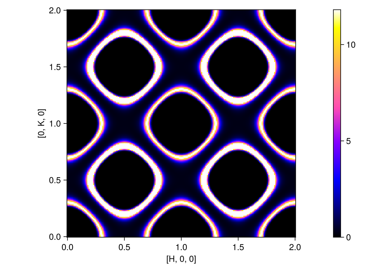

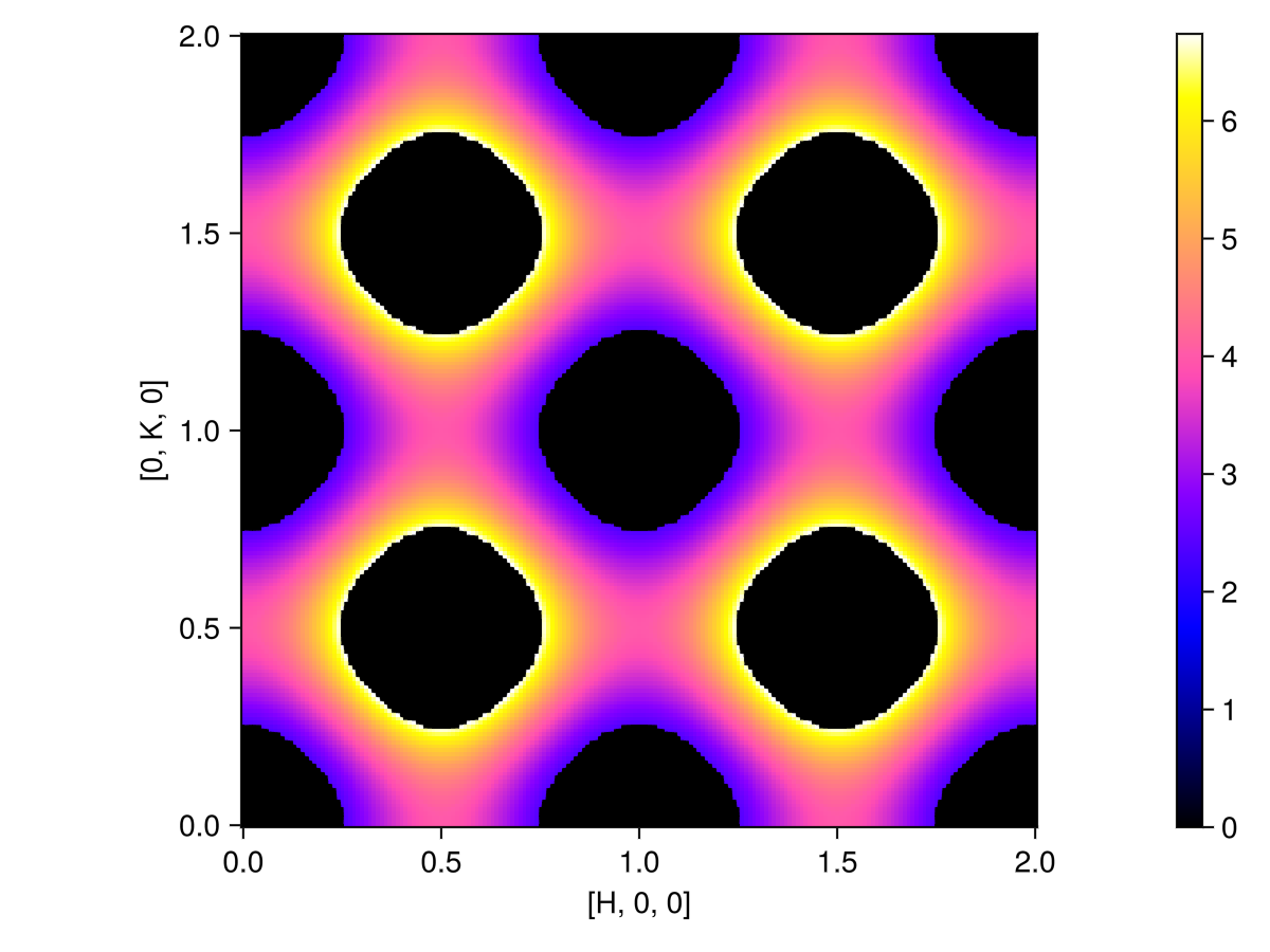
Integrate intensities between 3.5 and 4 meV using intensities_static with the bounds option.

res = intensities_static(swt, grid; bounds=(3.5, 4.01))
plot_intensities(res; units)