Download this example as Julia file or Jupyter notebook.

SW18 - Distorted kagome

This is a Sunny port of SpinW Tutorial 18, originally authored by Goran Nilsen and Sandor Toth. This tutorial illustrates spin wave calculations for KCu₃As₂O₇(OD)₃. The Cu ions are arranged in a distorted kagome lattice, and exhibit an incommensurate helical magnetic order, as described in G. J. Nilsen, et al., Phys. Rev. B 89, 140412 (2014). The model follows Toth and Lake, J. Phys.: Condens. Matter 27, 166002 (2015).

using Sunny, GLMakie

Build the distorted kagome crystal, with spacegroup 12.

units = Units(:meV, :angstrom)
latvecs = lattice_vectors(10.2, 5.94, 7.81, 90, 117.7, 90)
positions = [[0, 0, 0], [1/4, 1/4, 0]]
types = ["Cu1", "Cu2"]
cryst = Crystal(latvecs, positions, 12; types, setting="b1")
view_crystal(cryst)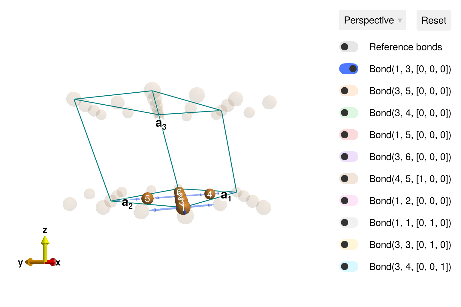

Define the interactions.

moments = [1 => Moment(s=1/2, g=2), 3 => Moment(s=1/2, g=2)]
sys = System(cryst, moments, :dipole, seed=0)
J   = -2
Jp  = -1
Jab = 0.75
Ja  = -J/.66 - Jab
Jip = 0.01
set_exchange!(sys, J, Bond(1, 3, [0, 0, 0]))
set_exchange!(sys, Jp, Bond(3, 5, [0, 0, 0]))
set_exchange!(sys, Ja, Bond(3, 4, [0, 0, 0]))
set_exchange!(sys, Jab, Bond(1, 2, [0, 0, 0]))
set_exchange!(sys, Jip, Bond(3, 4, [0, 0, 1]))

Use minimize_spiral_energy! to optimize the generalized spiral order. This determines the propagation wavevector k, and fits the spin values within the unit cell. One must provide a fixed axis perpendicular to the polarization plane. For this system, all interactions are rotationally invariant, and the axis vector is arbitrary. In other cases, a good axis will frequently be determined from symmetry considerations.

axis = [0, 0, 1]
randomize_spins!(sys)
k = minimize_spiral_energy!(sys, axis; k_guess=randn(3))
plot_spins(sys; ndims=2)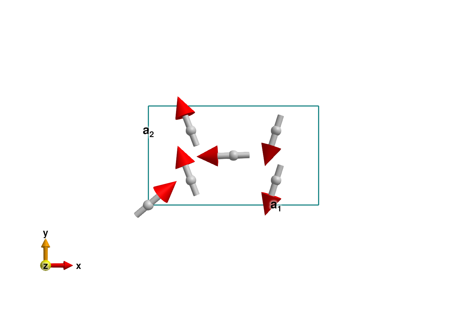

If successful, the optimization process will find one two propagation wavevectors, ±k_ref, with opposite chiralities. In this system, the spiral_energy_per_site is independent of chirality.

k_ref = [0.785902495, 0.0, 0.107048756]
k_ref_alt = [1, 0, 1] - k_ref
@assert isapprox(k, k_ref; atol=1e-6) || isapprox(k, k_ref_alt; atol=1e-6)
@assert spiral_energy_per_site(sys; k, axis) ≈ -0.78338383838

Check the energy with a real-space calculation using a large magnetic cell. First, we must determine a lattice size for which k becomes approximately commensurate.

suggest_magnetic_supercell([k_ref]; tol=1e-3)

Possible magnetic supercell in multiples of lattice vectors:

    [14 0 1; 0 1 0; 0 0 2]

for the rationalized wavevectors:

    [[11/14, 0, 3/28]]

Resize the system as suggested, and perform a real-space calculation. Working with a commensurate wavevector increases the energy slightly. The precise value might vary from run-to-run due to trapping in a local energy minimum.

new_shape = [14 0 1; 0 1 0; 0 0 2]
sys2 = reshape_supercell(sys, new_shape)
randomize_spins!(sys2)
minimize_energy!(sys2)
energy_per_site(sys2)

-0.7791966901275341

Return to the original system (with a single chemical cell) and construct SpinWaveTheorySpiral for calculations on the incommensurate spiral phase.

measure = ssf_perp(sys; apply_g=false)
swt = SpinWaveTheorySpiral(sys; measure, k, axis)

SpinWaveTheorySpiral(SpinWaveTheory(System([Dipole mode], Supercell (1×1×1)×6, Energy per site -0.3888), Sunny.SWTDataDipole(StaticArraysCore.SMatrix{3, 3, Float64, 9}[[0.5987703117069579 -0.5395540694904319 0.5919083712152307; -0.4397206527493308 0.3962338545106537 0.8060052605816745; -0.669417553821272 -0.7428863564744912 9.44302919362526e-10], [0.9863391001020876 -0.16000213433354427 0.039172651410326886; 0.03866719651386297 -0.006272522002614981 -0.9992324571297138; 0.16012503715397797 0.9870967391681716 2.634828523730855e-10], [0.16461316060429473 0.24210718470336132 0.9561833602771371; 0.5376273952850058 0.7907233411945912 -0.292768477690346; -0.8269578533365077 0.5622639138385771 1.3265775872409944e-8], [-0.008988914696491056 -0.3666147644035609 -0.9303294115171791; 0.02280357297768424 0.9300498970449665 -0.3667249460646208; 0.999699553101846 -0.024511293886068184 -1.2653244390977492e-8], [0.20943112855742355 0.20457757153441403 0.9561833608760643; 0.6840031172365236 0.6681514463255802 -0.2927684757342466; -0.6987691593093406 0.7153472317679836 1.4805023934753234e-8], [-0.08164484480782393 -0.35752105600238715 -0.9303294114620069; 0.20712141020967173 0.9069804492181744 -0.36672494620458473; 0.9749024775581725 -0.2226323409815756 -1.272128285472941e-8]], StaticArraysCore.SVector{3, Float64}[[0.5987703117069579, -0.5395540694904319, 0.5919083712152307] [0.9863391001020876, -0.16000213433354427, 0.039172651410326886] … [0.20943112855742355, 0.20457757153441403, 0.9561833608760643] [-0.08164484480782393, -0.35752105600238715, -0.9303294114620069]; [-0.4397206527493308, 0.3962338545106537, 0.8060052605816745] [0.03866719651386297, -0.006272522002614981, -0.9992324571297138] … [0.6840031172365236, 0.6681514463255802, -0.2927684757342466] [0.20712141020967173, 0.9069804492181744, -0.36672494620458473]; [-0.669417553821272, -0.7428863564744912, 9.44302919362526e-10] [0.16012503715397797, 0.9870967391681716, 2.634828523730855e-10] … [-0.6987691593093406, 0.7153472317679836, 1.4805023934753234e-8] [0.9749024775581725, -0.2226323409815756, -1.272128285472941e-8]], Sunny.StevensExpansion[Sunny.StevensExpansion(0, [0.0], [0.0, 0.0, 0.0, 0.0, 0.0], [0.0, 0.0, 0.0, 0.0, 0.0, 0.0, 0.0, 0.0, 0.0], [0.0, 0.0, 0.0, 0.0, 0.0, 0.0, 0.0, 0.0, 0.0, 0.0, 0.0, 0.0, 0.0]), Sunny.StevensExpansion(0, [0.0], [0.0, 0.0, 0.0, 0.0, 0.0], [0.0, 0.0, 0.0, 0.0, 0.0, 0.0, 0.0, 0.0, 0.0], [0.0, 0.0, 0.0, 0.0, 0.0, 0.0, 0.0, 0.0, 0.0, 0.0, 0.0, 0.0, 0.0]), Sunny.StevensExpansion(0, [0.0], [0.0, 0.0, 0.0, 0.0, 0.0], [0.0, 0.0, 0.0, 0.0, 0.0, 0.0, 0.0, 0.0, 0.0], [0.0, 0.0, 0.0, 0.0, 0.0, 0.0, 0.0, 0.0, 0.0, 0.0, 0.0, 0.0, 0.0]), Sunny.StevensExpansion(0, [0.0], [0.0, 0.0, 0.0, 0.0, 0.0], [0.0, 0.0, 0.0, 0.0, 0.0, 0.0, 0.0, 0.0, 0.0], [0.0, 0.0, 0.0, 0.0, 0.0, 0.0, 0.0, 0.0, 0.0, 0.0, 0.0, 0.0, 0.0]), Sunny.StevensExpansion(0, [0.0], [0.0, 0.0, 0.0, 0.0, 0.0], [0.0, 0.0, 0.0, 0.0, 0.0, 0.0, 0.0, 0.0, 0.0], [0.0, 0.0, 0.0, 0.0, 0.0, 0.0, 0.0, 0.0, 0.0, 0.0, 0.0, 0.0, 0.0]), Sunny.StevensExpansion(0, [0.0], [0.0, 0.0, 0.0, 0.0, 0.0], [0.0, 0.0, 0.0, 0.0, 0.0, 0.0, 0.0, 0.0, 0.0], [0.0, 0.0, 0.0, 0.0, 0.0, 0.0, 0.0, 0.0, 0.0, 0.0, 0.0, 0.0, 0.0])], [0.7071067811865476, 0.7071067811865476, 0.7071067811865476, 0.7071067811865476, 0.7071067811865476, 0.7071067811865476]), MeasureSpec, 1.0e-8), [0.21409750579919265, 4.198957025423508e-10, 0.8929512502032111], [0.0, 0.0, 1.0])

Plot intensities for a path through $𝐪$-space.

qs = [[0,0,0], [1,0,0]]
path = q_space_path(cryst, qs, 400)
res = intensities_bands(swt, path)
plot_intensities(res; units)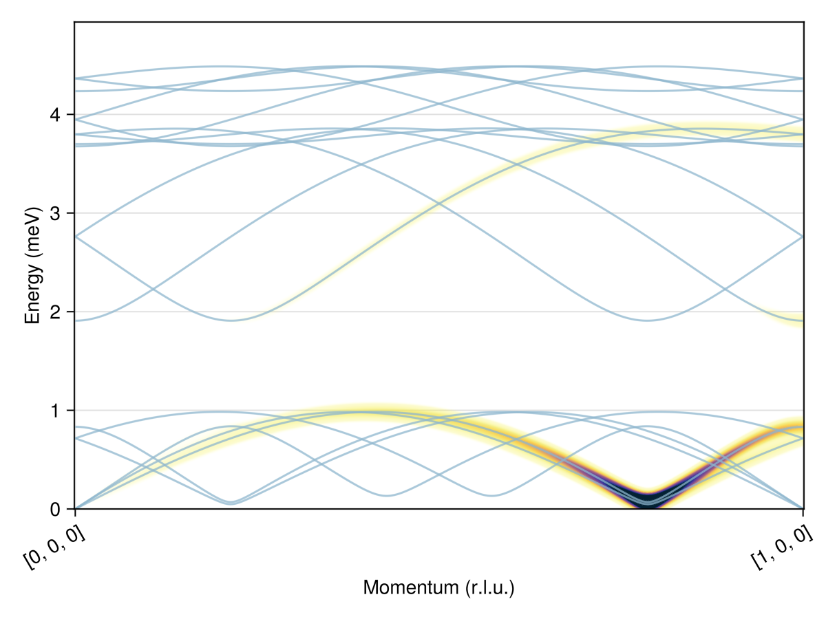

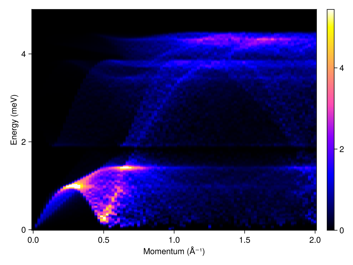
Plot the powder-averaged intensities

radii = range(0, 2, 100) # (1/Å)
energies = range(0, 6, 200)
kernel = gaussian(fwhm=0.05)
res = powder_average(cryst, radii, 400) do qs
    intensities(swt, qs; energies, kernel)
end
plot_intensities(res; units)