Download this example as Julia file or Jupyter notebook.
9. Disordered systems
This example uses SpinWaveTheoryKPM to efficiently calculate the neutron scattering spectrum of a disordered triangular antiferromagnet. The model is inspired by YbMgGaO4, as studied in Paddison et al, Nat. Phys., 13, 117–122 (2017) and Zhu et al, Phys. Rev. Lett. 119, 157201 (2017). Disordered occupancy of non-magnetic Mg/Ga sites can be modeled as a stochastic distribution of exchange constants and $g$-factors. Including this disorder introduces broadening of the spin wave spectrum.
using Sunny, GLMakieSet up minimal triangular lattice system. Include antiferromagnetic exchange interactions between nearest neighbor bonds. An optional seed for random number generation makes the calculations exactly reproducible on a fixed Julia version.
latvecs = lattice_vectors(1, 1, 10, 90, 90, 120)
cryst = Crystal(latvecs, [[0, 0, 0]])
sys = System(cryst, [1 => Moment(s=1/2, g=1)], :dipole; dims=(3, 3, 1), seed=0)
set_exchange!(sys, +1.0, Bond(1, 1, [1,0,0]))
Energy minimization yields the magnetic ground state with 120° angles between spins in triangular plaquettes.
randomize_spins!(sys)
minimize_energy!(sys)
plot_spins(sys; color=[S[3] for S in sys.dipoles], ndims=2)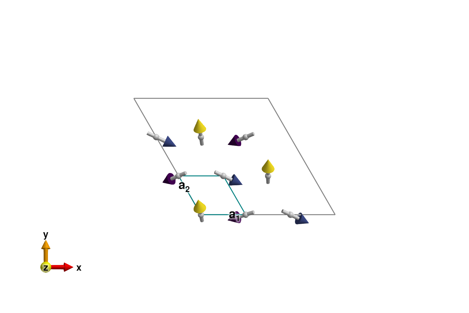
Select a $𝐪$-space path for the spin wave calculations.
qs = [[0, 0, 0], [1/3, 1/3, 0], [1/2, 0, 0], [0, 0, 0]]
labels = ["Γ", "K", "M", "Γ"]
path = q_space_path(cryst, qs, 150; labels)
QPath (150 samples)
Γ → K → M → Γ
Perform a traditional spin wave calculation. The spectrum shows sharp modes associated with coherent excitations about the K-point ordering wavevector, $𝐪 = [1/3, 1/3, 0]$.
kernel = lorentzian(fwhm=0.4)
energies = range(0.0, 3.0, 150)
swt = SpinWaveTheory(sys; measure=ssf_perp(sys))
res = intensities(swt, path; energies, kernel)
plot_intensities(res)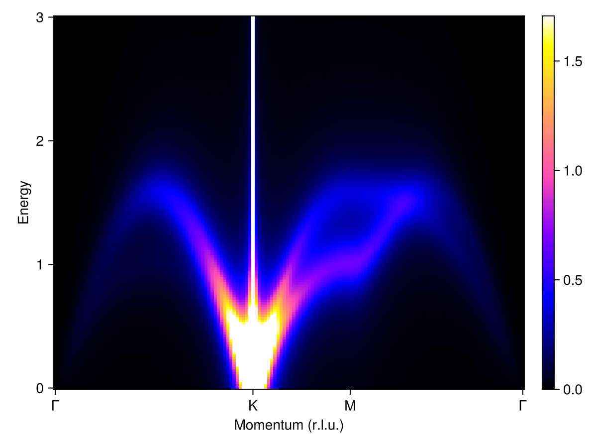
Use repeat_periodically to enlarge the system by a factor of 10 in each dimension. Use to_inhomogeneous to disable symmetry constraints and allow for the addition of disordered interactions.
sys_inhom = to_inhomogeneous(repeat_periodically(sys, (10, 10, 1)))System [Dipole mode]
Supercell (30×30×1)×1
Energy per site -3/8
Iterate over all symmetry_equivalent_bonds for nearest neighbor sites in the inhomogeneous system. Set the AFM exchange to include a noise term that has a standard deviation of 1/3. The newly minimized energy configuration allows for long wavelength modulations on top of the original 120° order.
for (site1, site2, offset) in symmetry_equivalent_bonds(sys_inhom, Bond(1, 1, [1, 0, 0]))
    noise = randn(sys_inhom.rng)/3
    set_exchange_at!(sys_inhom, 1.0 + noise, site1, site2; offset)
end

minimize_energy!(sys_inhom, maxiters=2_000)
plot_spins(sys_inhom; color=[S[3] for S in sys_inhom.dipoles], ndims=2)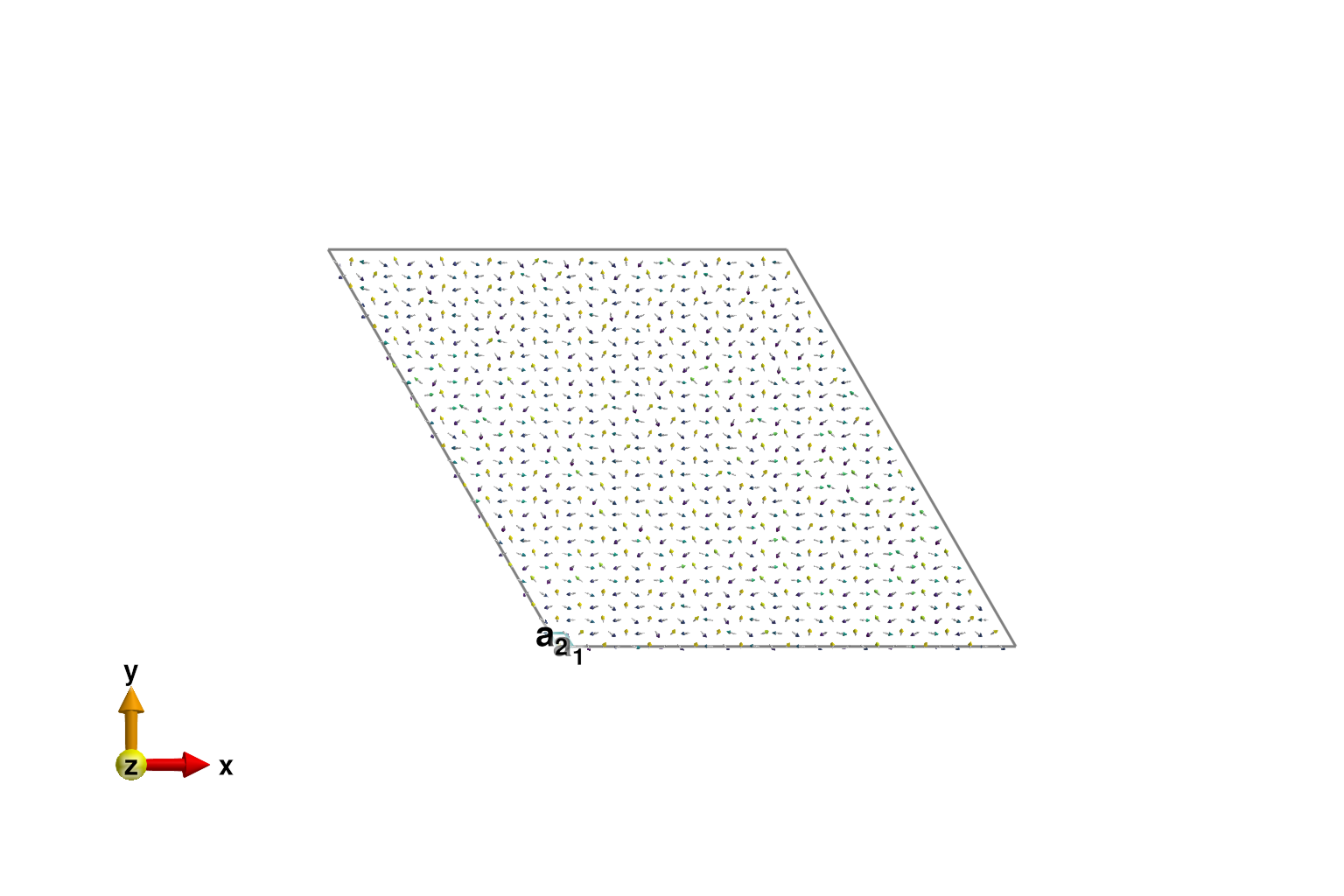
Traditional spin wave theory with exact diagonalization becomes impractical for large system sizes. Using SpinWaveTheoryKPM, the cost of an intensities calculation becomes linear in the system size, with a prefactor that inversely in the width of the line broadening kernel. Good choices for the dimensionless error tolerance are tol=0.05 (more speed) or tol=0.01 (more accuracy).
Observe that disorder in the nearest-neighbor exchange serves to broaden the discrete excitation bands into a continuum.
swt = SpinWaveTheoryKPM(sys_inhom; measure=ssf_perp(sys_inhom), tol=0.05)
res = intensities(swt, path; energies, kernel)
plot_intensities(res)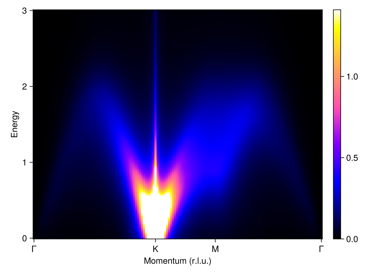
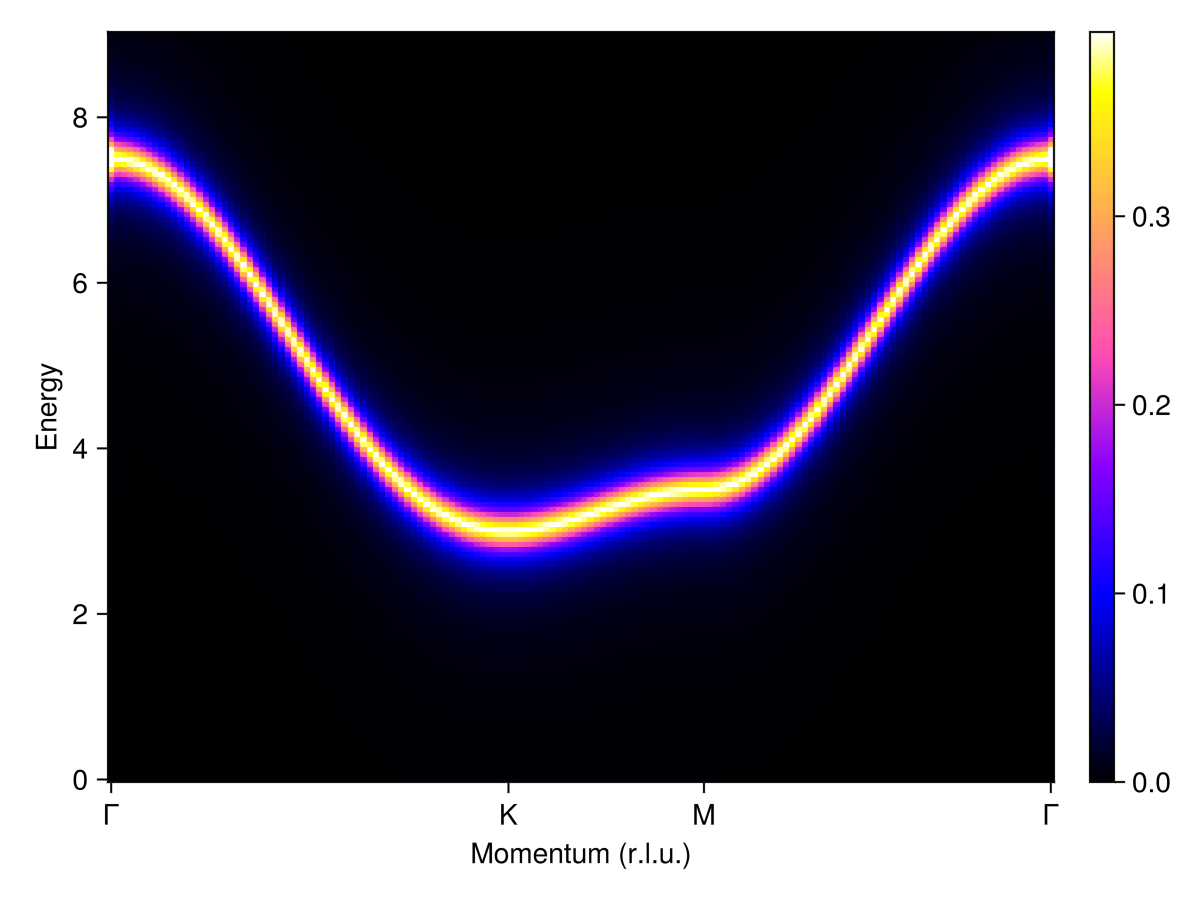
Now apply a magnetic field of magnitude 7.5 (energy units) along the global $ẑ$ axis. This field fully polarizes the spins and opens a gap. The spin wave spectrum shows a sharp mode at the Γ-point (zone center) that broadens into a continuum along the K and M points (zone boundary).
set_field!(sys_inhom, [0, 0, 7.5])
randomize_spins!(sys_inhom)
minimize_energy!(sys_inhom)

energies = range(0.0, 9.0, 150)
swt = SpinWaveTheoryKPM(sys_inhom; measure=ssf_perp(sys_inhom), tol=0.05)
res = intensities(swt, path; energies, kernel)
plot_intensities(res)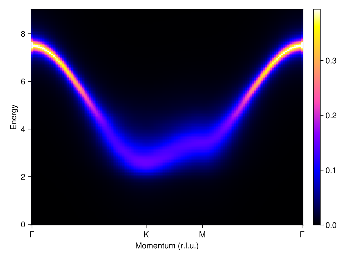
Add disorder to the $z$-component of each magnetic moment $g$-tensor. This further broadens intensities, now across the entire path. Some intensity modulation within the continuum is also apparent. This modulation is a finite-size effect and would be mitigated by enlarging the system beyond 30×30 chemical cells.
for site in eachsite(sys_inhom)
    noise = randn(sys_inhom.rng)/6
    sys_inhom.gs[site] = [1 0 0; 0 1 0; 0 0 1+noise]
end
randomize_spins!(sys_inhom)
minimize_energy!(sys_inhom)

swt = SpinWaveTheoryKPM(sys_inhom; measure=ssf_perp(sys_inhom), tol=0.05)
res = intensities(swt, path; energies, kernel)
plot_intensities(res)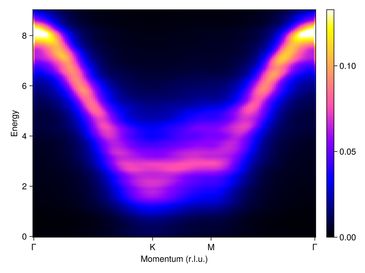
For reference, the equivalent non-disordered system shows a single coherent mode.
set_field!(sys, [0, 0, 7.5])
randomize_spins!(sys)
minimize_energy!(sys)
swt = SpinWaveTheory(sys; measure=ssf_perp(sys))
res = intensities(swt, path; energies, kernel)
plot_intensities(res)