Download this example as Julia file or Jupyter notebook.

2. Landau-Lifshitz dynamics of CoRh₂O₄ at finite T

In the previous tutorial, we used spin wave theory to calculate the dynamical spin structure factor of CoRh₂O₄. Here, we perform a similar calculation using equilibrium samples from the Boltzmann distribution at finite $T$. For each sampled spin configuration, we will simulate the classical Landau-Lifshitz spin dynamics and extract dynamical spin-spin correlations. After applying a classical-to-quantum correction factor, the resulting intensities can be compared to inelastic neutron scattering data.

Construct the system as in the previous tutorial. For this antiferromagnetic model on the diamond cubic lattice, the ground state is unfrustrated Néel order.

using Sunny, GLMakie

units = Units(:meV, :angstrom)
a = 8.5031 # (Å)
latvecs = lattice_vectors(a, a, a, 90, 90, 90)
cryst = Crystal(latvecs, [[0,0,0]], 227, setting="1")

sys = System(cryst, [1 => Moment(s=3/2, g=2)], :dipole)
J = 0.63 # (meV)
set_exchange!(sys, J, Bond(1, 3, [0,0,0]))
randomize_spins!(sys)
minimize_energy!(sys)
plot_spins(sys; color=[S[3] for S in sys.dipoles])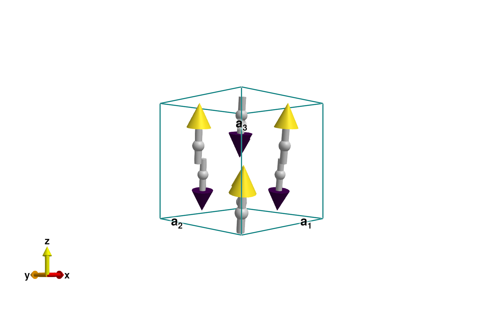

Use repeat_periodically to extend the system to 10×10×10 chemical unit cells. The ground state Néel order is retained. Increasing the system size further would reduce finite-size artifacts and increase momentum-space resolution, but would also make the simulations slower.

sys = repeat_periodically(sys, (10, 10, 10))
plot_spins(sys; color=[S[3] for S in sys.dipoles])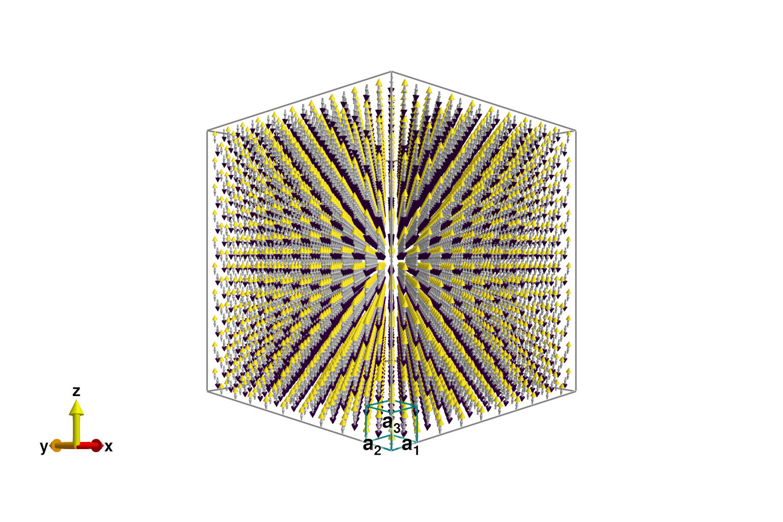

Langevin dynamics for sampling

We will be using a Langevin spin dynamics to thermalize the system. This dynamics is a variant of the Landau-Lifshitz equation that incorporates noise and dissipation terms, which are linked by a fluctuation-dissipation theorem. The temperature 6 K ≈ 1.38 meV is slightly above ordering for this model. The dimensionless damping magnitude sets a timescale for coupling to the implicit thermal bath; 0.2 is usually a good choice.

langevin = Langevin(; damping=0.2, kT=16*units.K)

Langevin(<missing>; damping=0.2, kT=1.3787733219432283)

Use suggest_timestep to select an integration timestep. A dimensionless error tolerance of 1e-2 is usually a good choice. The suggested timestep will vary according to the magnetic configuration. It is reasonable to start from an energy-minimized configuration.

suggest_timestep(sys, langevin; tol=1e-2)
langevin.dt = 0.025;

Consider dt ≈ 0.02528 for this spin configuration at tol = 0.01.

Now run a Langevin trajectory to sample spin configurations. Keep track of the energy per site at each time step.

energies = [energy_per_site(sys)]
for _ in 1:1000
    step!(sys, langevin)
    push!(energies, energy_per_site(sys))
end

From the relaxed spin configuration, we can learn that dt was a little smaller than necessary; increasing it will make the remaining simulations faster.

suggest_timestep(sys, langevin; tol=1e-2)
langevin.dt = 0.042;

Consider dt ≈ 0.04159 for this spin configuration at tol = 0.01. Current value is dt = 0.025.

Plot energy versus time using the Makie lines function. The plateau suggests that the system has reached thermal equilibrium.

lines(energies, color=:blue, figure=(size=(600,300),), axis=(xlabel="Timesteps", ylabel="Energy (meV)"))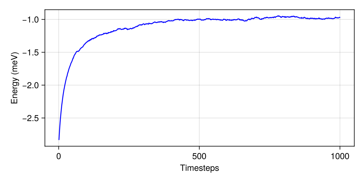

Plot the spins colored by their alignment with a reference spin at the origin. The field sys.dipoles is a 4D array storing the spin dipole data. The first three indices of label the chemical cell, while the fourth index labels an atom within the cell. Note that Julia arrays use 1-based indexing. Thermal fluctuations are apparent in the plot.

S0 = sys.dipoles[1,1,1,1]
plot_spins(sys; color=[S'*S0 for S in sys.dipoles])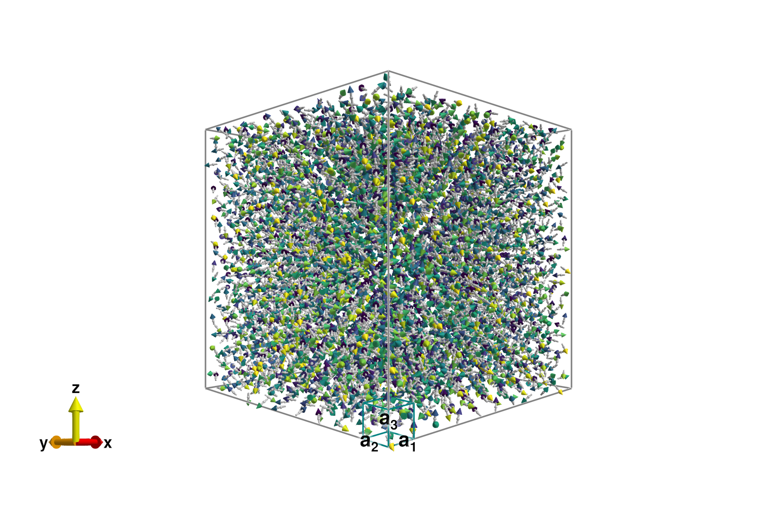

Static structure factor

Use SampledCorrelationsStatic to estimate spatial correlations for configurations in classical thermal equilibrium. Each call to add_sample! will accumulate data for the current spin snapshot.

formfactors = [1 => FormFactor("Co2")]
measure = ssf_perp(sys; formfactors)
sc = SampledCorrelationsStatic(sys; measure)
add_sample!(sc, sys)    # Accumulate the newly sampled structure factor into `sf`

Collect 20 additional samples. Perform 100 Langevin time-steps between measurements to approximately decorrelate the sample in thermal equilibrium.

for _ in 1:20
    for _ in 1:100
        step!(sys, langevin)
    end
    add_sample!(sc, sys)
end

Use q_space_grid to define a slice of momentum space $[H, K, 0]$, where $H$ and $K$ each range from -10 to 10 in RLU. This command produces a 200×200 grid of sample points.

grid = q_space_grid(cryst, [1, 0, 0], range(-10, 10, 200), [0, 1, 0], (-10, 10))

Sunny.QGrid{2} (200×200 samples)

Calculate and plot the instantaneous structure factor on the slice by integrating over all energy values ω. We employ the appropriate FormFactor for Co2⁺. Selecting saturation = 1.0 sets the color saturation point to the maximum intensity value. This is reasonable because we are above the ordering temperature, and do not have sharp Bragg peaks.

res = intensities_static(sc, grid)
plot_intensities(res; saturation=1.0, title="Static Intensities at T = 16 K")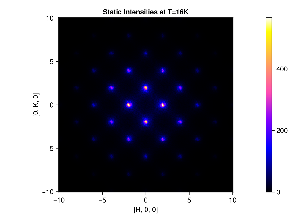

Dynamical structure factor

To collect statistics for the dynamical structure factor intensities $\mathcal{S}(𝐪,ω)$ at finite temperature, use SampledCorrelations. It requires a range of energies to resolve, which will be associated with frequencies of the classical spin dynamics. The integration timestep dt can be somewhat larger than that used by the Langevin dynamics.

dt = 2*langevin.dt
energies = range(0, 6, 50)
sc = SampledCorrelations(sys; dt, energies, measure=ssf_perp(sys))

SampledCorrelations (612.974 MiB)
[S(q,ω) | nω = 49, Δω = 0.1224 | 0 sample]
Lattice: (3,) × 8

Like before, use Langevin dynamics to sample spin configurations from thermal equilibrium. Now, however, each call to add_sample! will run a classical spin dynamics trajectory and measure dynamical correlations. To make the tutorial run quickly, we average over just 5 trajectories. To make a publication quality figure, this number should be significantly increased for better statistics.

for _ in 1:5
    for _ in 1:100
        step!(sys, langevin)
    end
    add_sample!(sc, sys)
end

Select points that define a piecewise-linear path through reciprocal space, and a sampling density.

qs = [[3/4, 3/4,   0],
      [  0,   0,   0],
      [  0, 1/2, 1/2],
      [1/2,   1,   0],
      [  0,   1,   0],
      [1/4,   1, 1/4],
      [  0,   1,   0],
      [  0,  -4,   0]]
path = q_space_path(cryst, qs, 500)

QPath (500 samples)
  [3/4, 3/4, 0] → [0, 0, 0] → [0, 1/2, 1/2] → [1/2, 1, 0] → [0, 1, 0] → [1/4, 1, 1/4] → [0, 1, 0] → [0, -4, 0]

Calculate and plot the intensities along this path.

res = intensities(sc, path; energies, langevin.kT)
plot_intensities(res; units, title="Intensities at 16 K")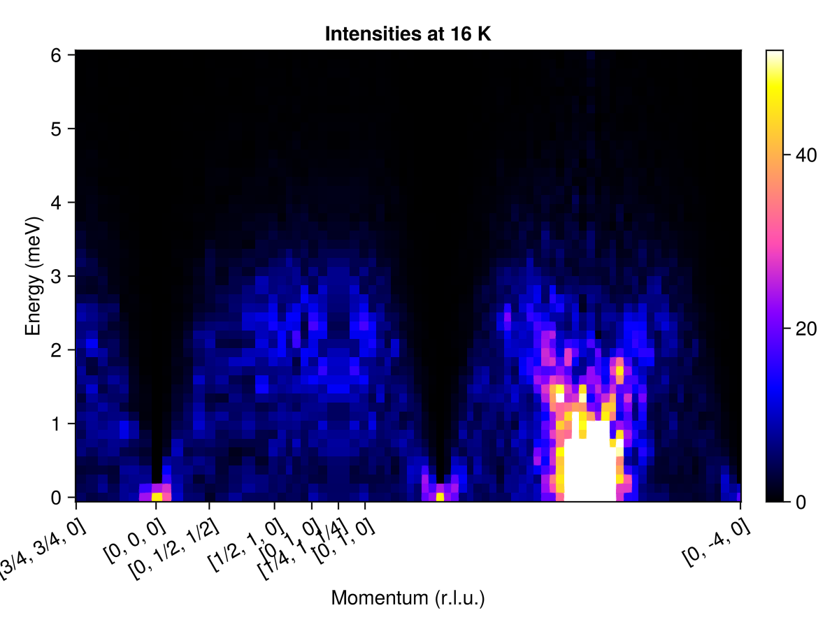

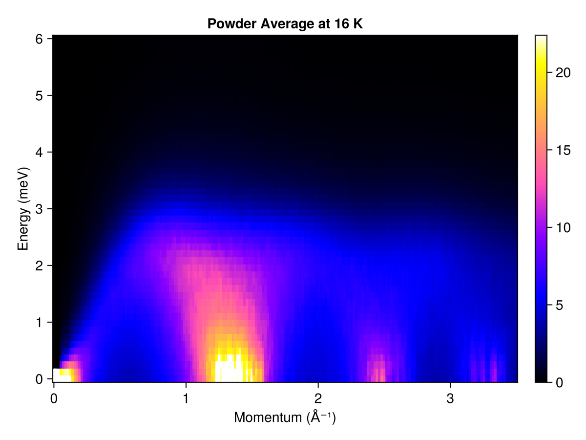
Powder averaged intensity

Define spherical shells in reciprocal space via their radii, in absolute units of 1/Å. For each shell, calculate and average the intensities at 350 $𝐪$-points

radii = range(0, 3.5, 200) # (1/Å)
res = powder_average(cryst, radii, 350) do qs
    intensities(sc, qs; energies, langevin.kT)
end
plot_intensities(res; units, title="Powder Average at 16 K")