Download this example as Julia file or Jupyter notebook.
SW08 - √3×√3 kagome antiferromagnet
This is a Sunny port of SpinW Tutorial 8, originally authored by Bjorn Fak and Sandor Toth. It calculates the linear spin wave theory spectrum for the $\sqrt{3} \times \sqrt{3}$ order of a kagome antiferromagnet.
Load Sunny and the GLMakie plotting package.
using Sunny, GLMakieDefine the chemical cell of a kagome lattice with spacegroup 147 (P-3).
units = Units(:meV, :angstrom)
latvecs = lattice_vectors(6, 6, 40, 90, 90, 120)
cryst = Crystal(latvecs, [[1/2, 0, 0]], 147)
view_crystal(cryst; ndims=2)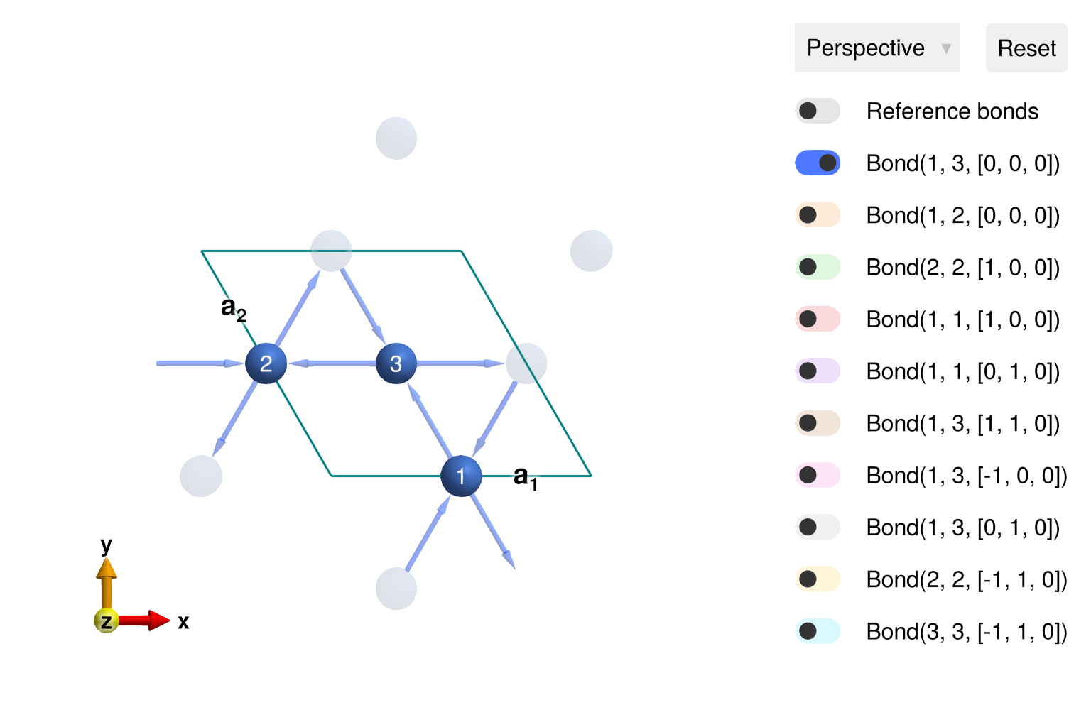
Construct a spin system with nearest neighbor antiferromagnetic exchange.
sys = System(cryst, [1 => Moment(s=1, g=2)], :dipole)
J = 1.0
set_exchange!(sys, J, Bond(2, 3, [0, 0, 0]))
Initialize to an energy minimizing magnetic structure, for which nearest-neighbor spins are at 120° angles.
set_dipole!(sys, [cos(0), sin(0), 0], (1, 1, 1, 1))
set_dipole!(sys, [cos(0), sin(0), 0], (1, 1, 1, 2))
set_dipole!(sys, [cos(2π/3), sin(2π/3), 0], (1, 1, 1, 3))
k = [-1/3, -1/3, 0]
axis = [0, 0, 1]
sys_enlarged = repeat_periodically_as_spiral(sys, (3, 3, 1); k, axis)
plot_spins(sys_enlarged; ndims=2)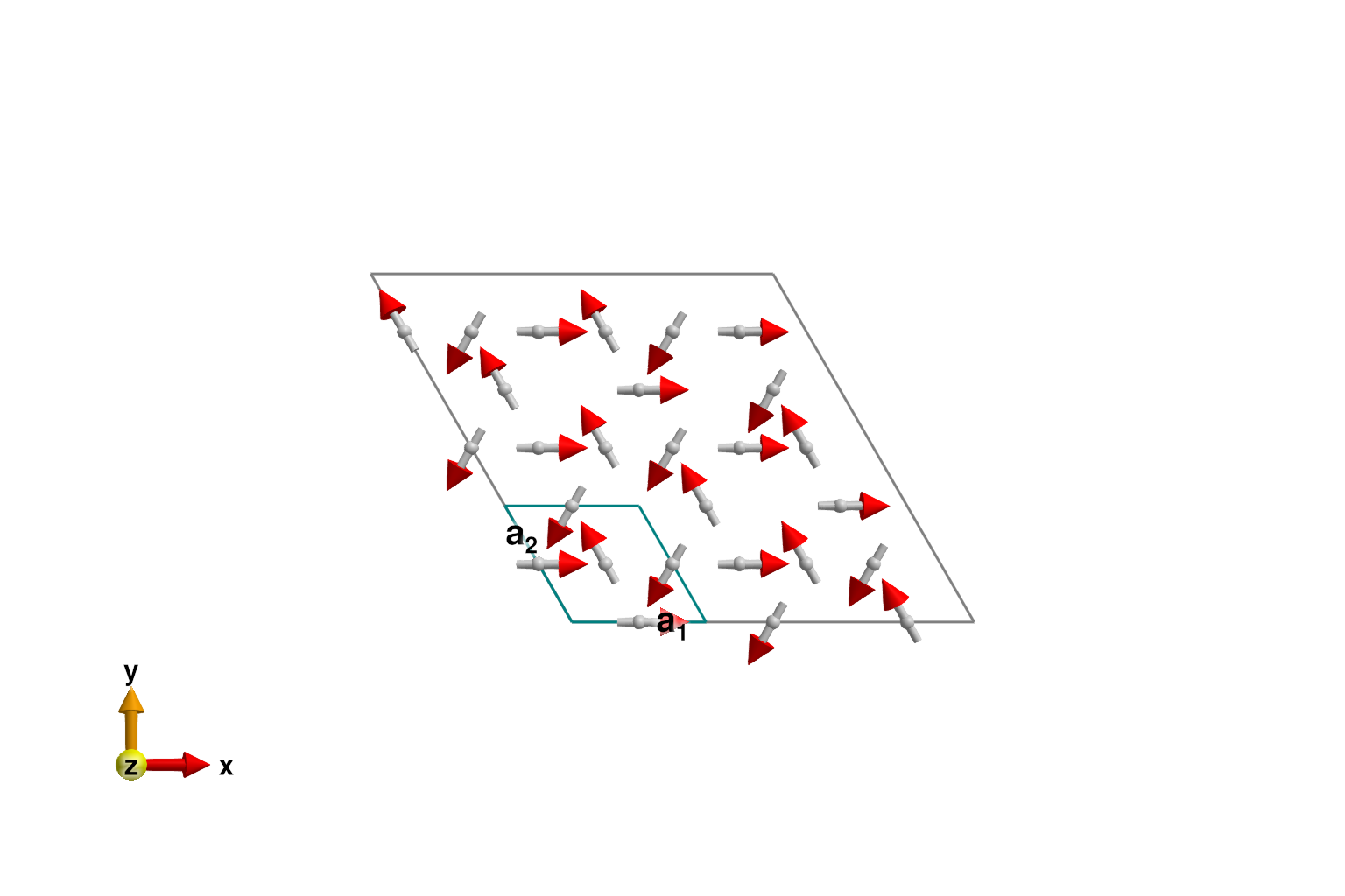
Check energy per site. Each site participates in 4 bonds with energy $J\cos(2π/3)$. Factor of 1/2 avoids double counting. The two calculation methods agree.
@assert energy_per_site(sys_enlarged) ≈ (4/2)*J*cos(2π/3)
@assert spiral_energy_per_site(sys; k, axis) ≈ (4/2)*J*cos(2π/3)
Calculate and plot intensities for a path through $𝐪$-space using two calculation methods. The two methods agree in intensity, but the "supercell method" gives rise to ghost modes in the dispersion that have zero intensity.
qs = [[-1/2,0,0], [0,0,0], [1/2,1/2,0]]
path = q_space_path(cryst, qs, 400)

fig = Figure(size=(768, 300))
swt = SpinWaveTheory(sys_enlarged; measure=ssf_perp(sys_enlarged))
res = intensities_bands(swt, path)
plot_intensities!(fig[1, 1], res; units, saturation=0.5,title="Supercell method")
swt = SpinWaveTheorySpiral(sys; measure=ssf_perp(sys), k, axis)
res = intensities_bands(swt, path)
plot_intensities!(fig[1, 2], res; units, saturation=0.5, title="Spiral method")
fig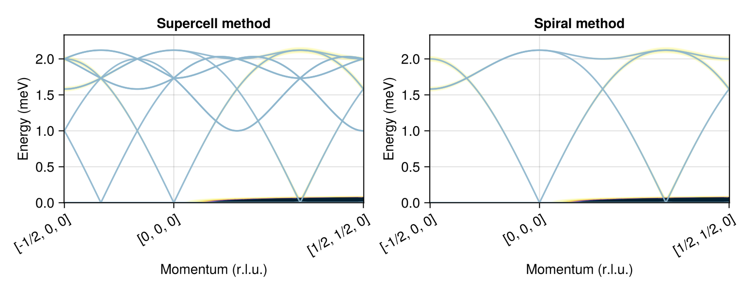
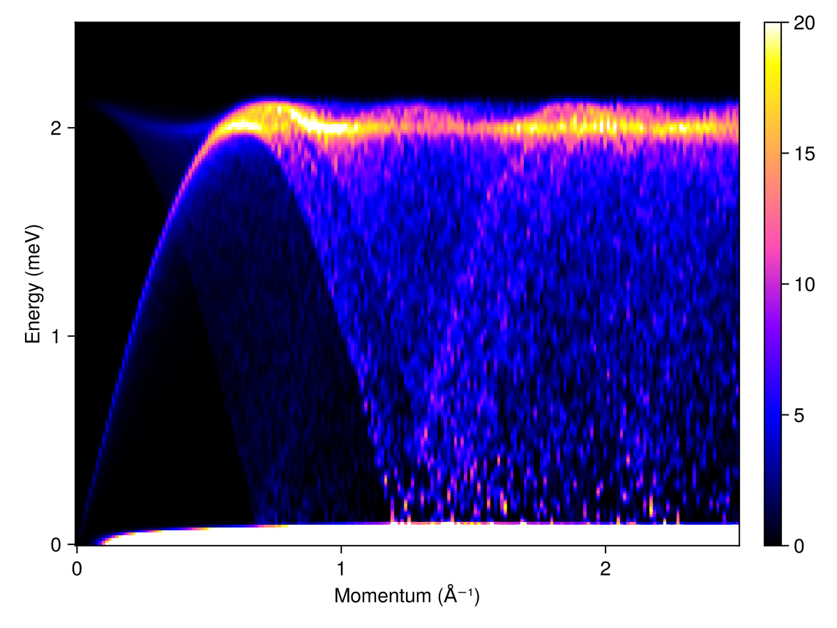
Calculate and plot the powder averaged spectrum. Continuing to use the "spiral method", this calculation executes in about two seconds. Because the intensities are dominated by a flat band at zero energy transfer, select an empirical colorrange that brings the lower-intensity features into focus.
radii = range(0, 2.5, 200)
energies = range(0, 2.5, 200)
kernel = gaussian(fwhm=0.05)
res = powder_average(cryst, radii, 200) do qs
    intensities(swt, qs; energies, kernel)
end
plot_intensities(res; units, colorrange=(0, 20))