Download this example as Julia file or Jupyter notebook.

SW19 - Different magnetic ions

This is a Sunny port of SpinW Tutorial 19, originally authored by Bjorn Fak and Sandor Toth. This tutorial illustrates how to eliminate magnetic contributions from a subset of ions via the special value zero(FormFactor).

using Sunny, GLMakie

Build a crystal with Cu²⁺ and Fe²⁺ ions.

units = Units(:meV, :angstrom)
a = 3.0
b = 8.0
c = 4.0
latvecs = lattice_vectors(a, b, c, 90, 90, 90)
positions = [[0, 0, 0], [0, 1/2, 0]]
types = ["Cu2", "Fe2"]
cryst = Crystal(latvecs, positions, 1; types)
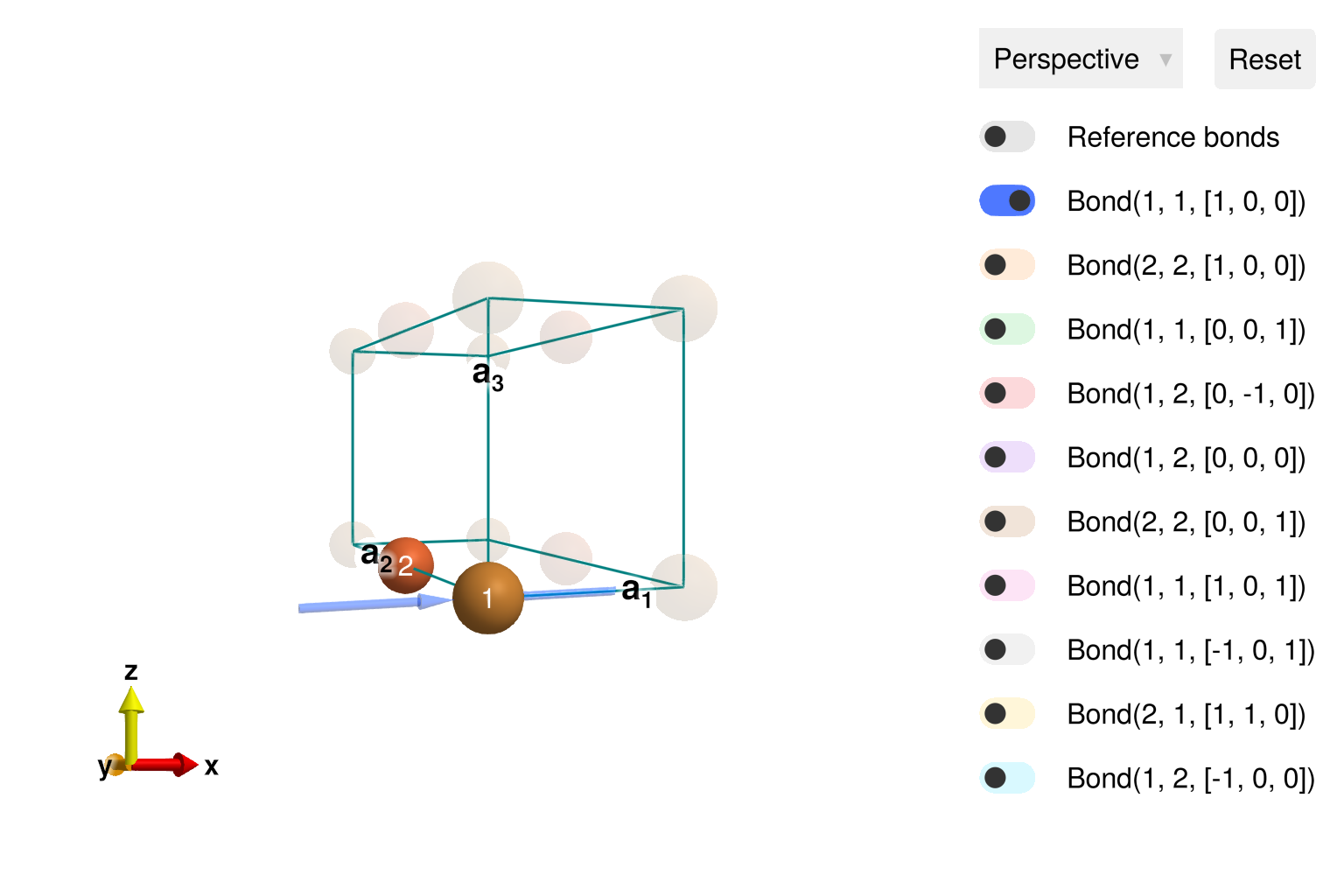
view_crystal(cryst)

Set exchange interactions.

J_Cu_Cu = 1.0
J_Fe_Fe = 1.0
J_Cu_Fe = -0.1
moments = [1 => Moment(s=1/2, g=2), 2 => Moment(s=2, g=2)]
sys = System(cryst, moments, :dipole; dims=(2, 1, 1))
set_exchange!(sys, J_Cu_Cu, Bond(1, 1, [-1, 0, 0]))
set_exchange!(sys, J_Fe_Fe, Bond(2, 2, [-1, 0, 0]))
set_exchange!(sys, J_Cu_Fe, Bond(2, 1, [0, 1, 0]))
set_exchange!(sys, J_Cu_Fe, Bond(1, 2, [0, 0, 0]))

Find and plot a minimum energy configuration.

randomize_spins!(sys)
minimize_energy!(sys)
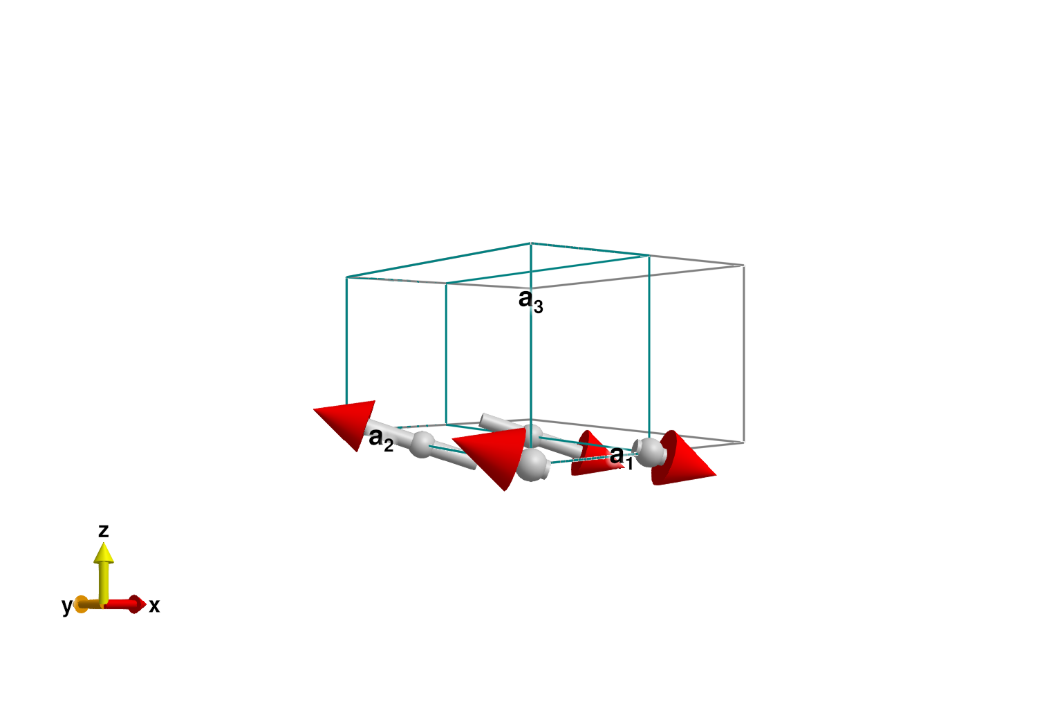
plot_spins(sys)

Define a path through $𝐪$-space.

qs = [[0,0,0], [1,0,0]]
path = q_space_path(cryst, qs, 400)

QPath (400 samples)
  [0, 0, 0] → [1, 0, 0]

Plot different pair correlation intensities by varying the FormFactor on different atom types. Indices 1 and 2 refer to atoms in the original chemical, and are propagated by symmetry. The special "zero" form factor effectively removes the spin moment from the calculation.

fig = Figure(size=(768,600))

formfactors = [1 => FormFactor("Cu2"), 2 => FormFactor("Fe2")]
swt = SpinWaveTheory(sys; measure=ssf_trace(sys; formfactors))
res = intensities_bands(swt, path)
plot_intensities!(fig[1, 1], res; units, title="All correlations")

formfactors = [1 => FormFactor("Cu2"), 2 => zero(FormFactor)]
swt = SpinWaveTheory(sys; measure=ssf_trace(sys; formfactors))
res = intensities_bands(swt, path)
plot_intensities!(fig[1, 2], res; units, title="Cu-Cu correlations")

formfactors = [1 => zero(FormFactor), 2 => FormFactor("Fe2")]
swt = SpinWaveTheory(sys; measure=ssf_trace(sys; formfactors))
res = intensities_bands(swt, path)
plot_intensities!(fig[2, 2], res; units, title="Fe-Fe correlations")

fig

Calculate quantum corrections $δS$ to spin magnitude, which arise from the zero-point energy of the spin waves. The outputs are ordered following the Site indexing scheme for the system sys: (cell1, cell2, cell3, sublattice), with left-most indices fastest. The two corrections $δS ≈ -0.137$ and $δS ≈ -0.578$ apply to the Cu and Fe ions, respectively. The larger correction on Fe is due to the relatively weak interchain coupling.

Sunny.magnetization_lswt_correction_dipole(swt; atol=1e-4)

4-element StaticArraysCore.SVector{4, Float64} with indices SOneTo(4):
 -0.13698215962703128
 -0.13698215962697904
 -0.5783052943276753
 -0.5783052943274667