Download this example as Julia file or Jupyter notebook.
SW06 - Complex kagome ferromagnet
This is a Sunny port of SpinW Tutorial 6, originally authored by Bjorn Fak and Sandor Toth. It calculates the spin wave spectrum of the kagome lattice with multiple competing interactions.
Load Sunny and the GLMakie plotting package.
using Sunny, GLMakieDefine the chemical cell of a kagome lattice with spacegroup 147 (P-3).
units = Units(:meV, :angstrom)
latvecs = lattice_vectors(6, 6, 8, 90, 90, 120)
cryst = Crystal(latvecs, [[1/2, 0, 0]], 147)
view_crystal(cryst; ndims=2)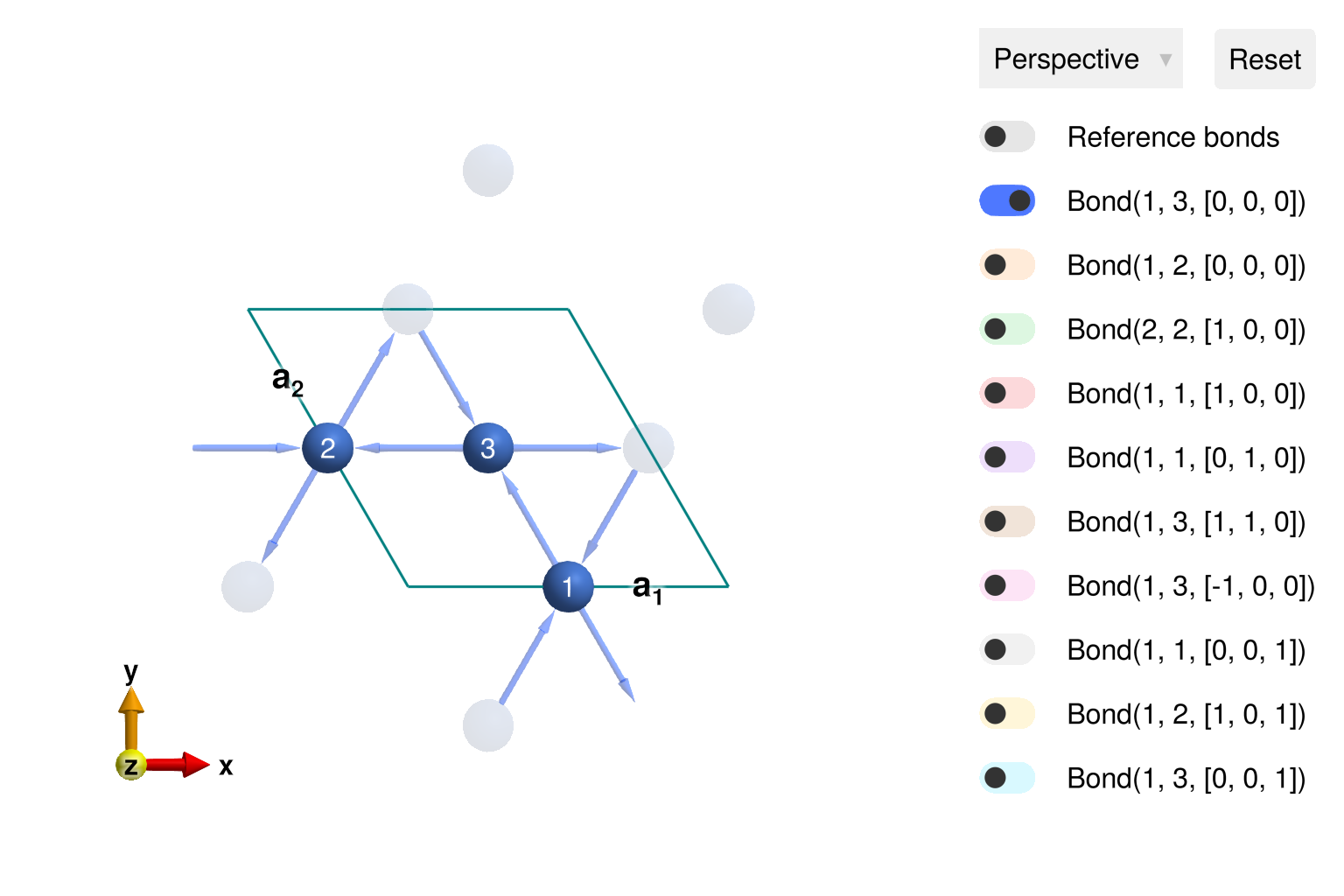
Construct a spin system with strongly ferromagnetic nearest-neighbor interactions, and two additional interactions. There are two symmetry-inequivalent exchange types at distance 6 Å (3rd nearest neighbor). The first type, associated with J3a, is a bond from atom 2 to atom 2 that passes over atom 3. The second type, associated with J3b, is a bond from atom 1 to atom 1 that passes through the center of an "empty" hexagon of the kagome lattice.
sys = System(cryst, [1 => Moment(s=1, g=2)], :dipole)
J1 = -1.0
J2 = 0.1
J3a = 0.00
J3b = 0.17
set_exchange!(sys, J1, Bond(2, 3, [0, 0, 0]))
set_exchange!(sys, J2, Bond(2, 1, [0, 0, 0]))
set_exchange!(sys, J3a, Bond(2, 2, [1, 0, 0]))
set_exchange!(sys, J3b, Bond(1, 1, [1, 0, 0]))
Interactively visualize the specified interactions. Red (blue) color indicates FM (AFM).
view_crystal(sys; ndims=2)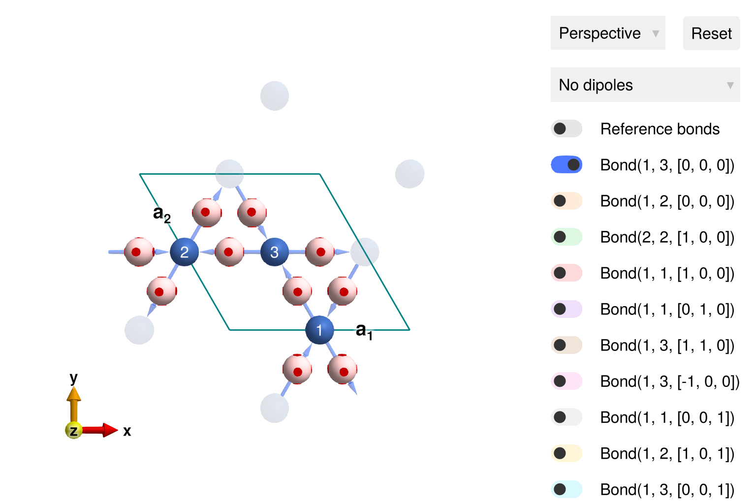
Energy minimization favors ferromagnetic order.
randomize_spins!(sys)
minimize_energy!(sys)
plot_spins(sys; ndims=2)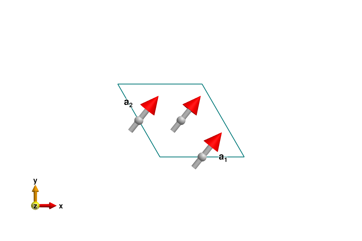
Calculate and plot intensities for a path through $𝐪$-space.
swt = SpinWaveTheory(sys; measure=ssf_perp(sys))
qs = [[-1/2,0,0], [0,0,0], [1/2,1/2,0]]
path = q_space_path(cryst, qs, 400)
res = intensities_bands(swt, path)
plot_intensities(res; units)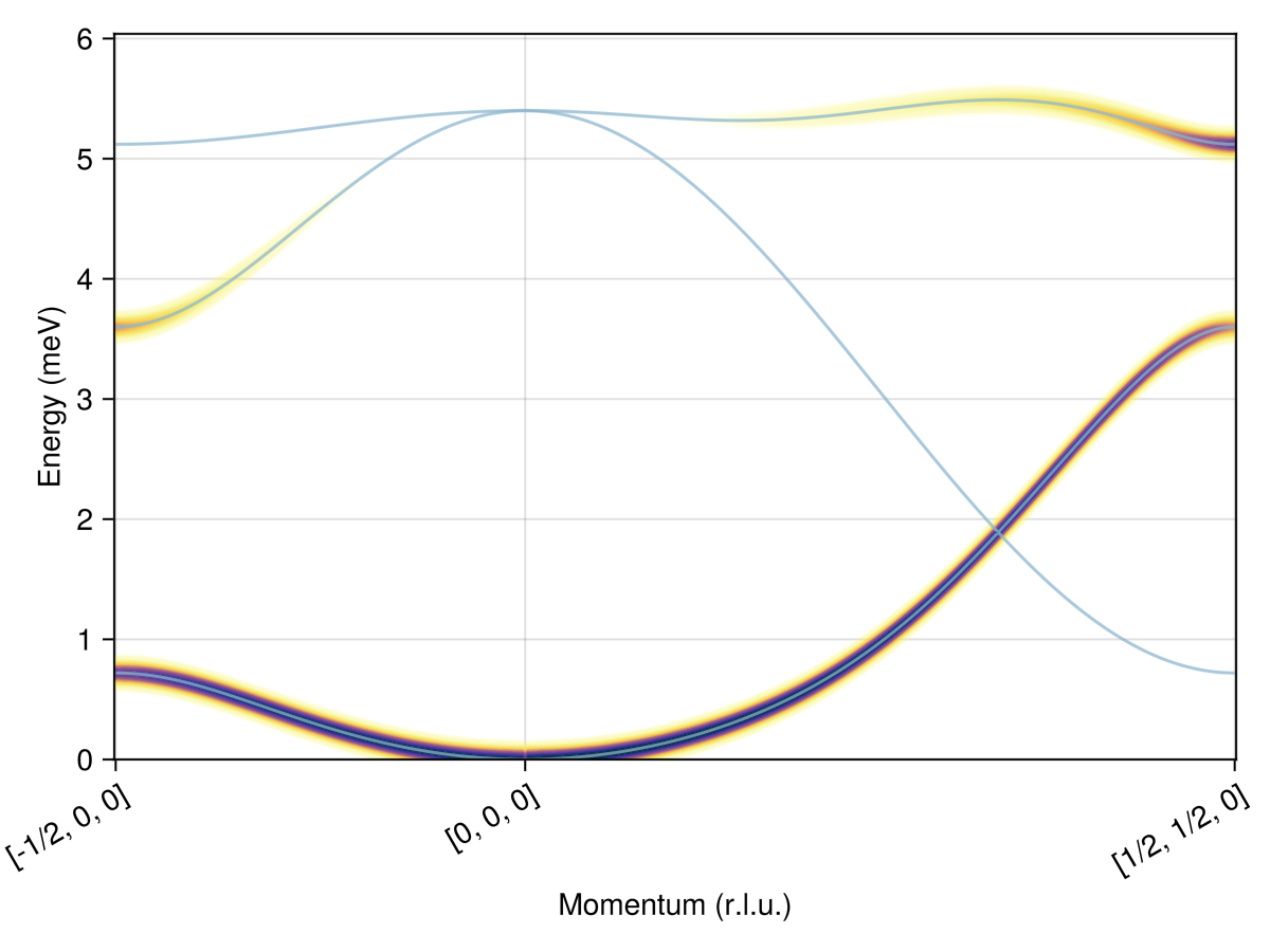
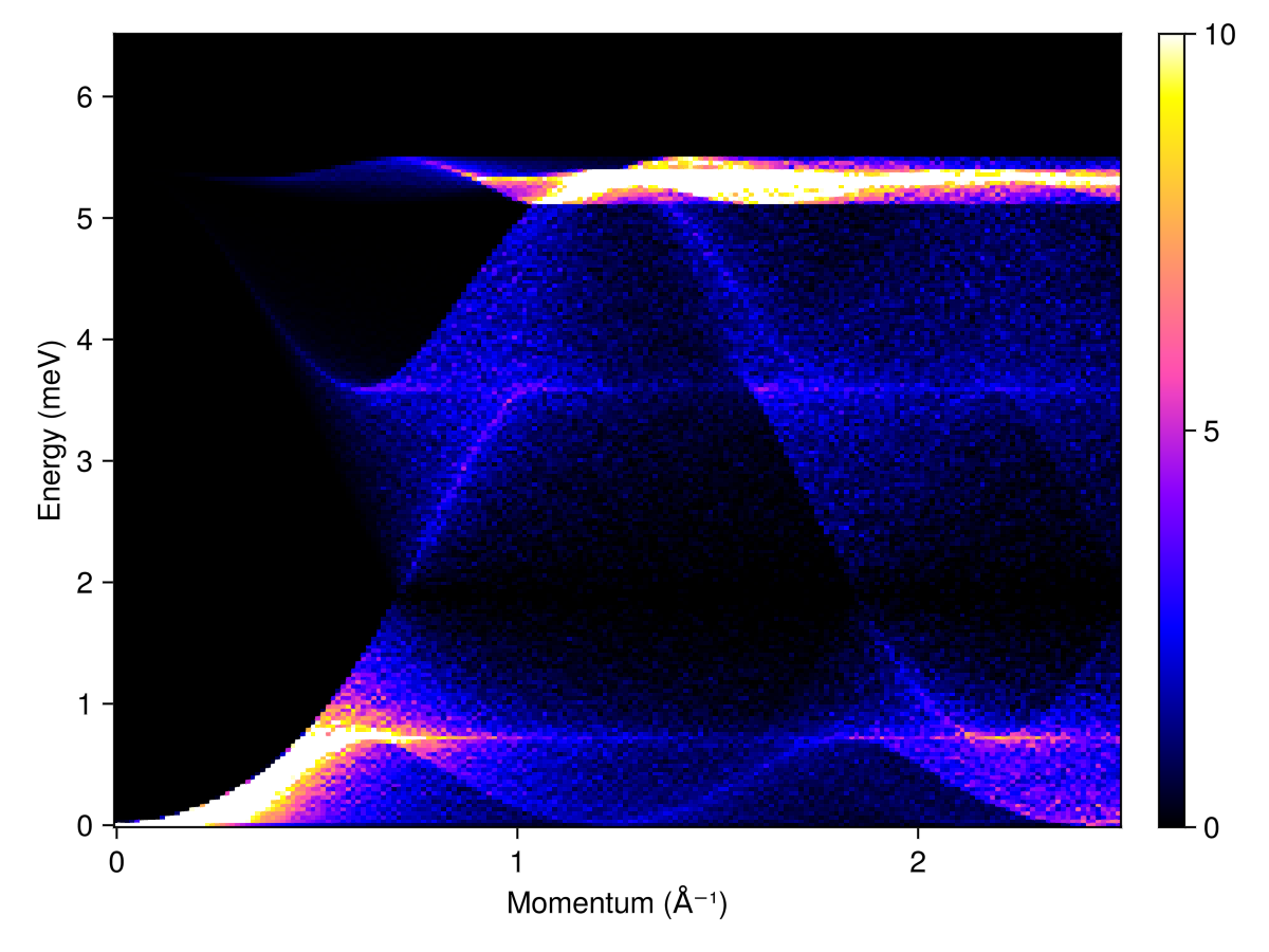
Calculate and plot the powder averaged spectrum. Select an empirical colorrange that brings the lower-intensity features into focus.
radii = range(0, 2.5, 200)
energies = range(0, 6.5, 200)
kernel = gaussian(fwhm=0.02)
res = powder_average(cryst, radii, 1000) do qs
    intensities(swt, qs; energies, kernel)
end
plot_intensities(res; units, colorrange=(0,10))