Download this example as Julia file or Jupyter notebook.

SW14 - YVO₃

This is a Sunny port of SpinW Tutorial 14, originally authored by Sandor Toth. It calculates the spin wave spectrum of YVO₃.

Load packages

using Sunny, GLMakie

Build an orthorhombic lattice and populate the V atoms according to the pseudocubic unit cell, doubled along the c-axis. The listed spacegroup of the YVO₃ chemical cell is international number 62. It has been observed, however, that the exchange interactions break this symmetry. For this reason, disable all symmetry analysis by selecting spacegroup 1 (P1).

units = Units(:meV, :angstrom)
a = 5.2821 / sqrt(2)
b = 5.6144 / sqrt(2)
c = 7.5283
latvecs = lattice_vectors(a, b, c, 90, 90, 90)
positions = [[0, 0, 0], [0, 0, 1/2]]
types = ["V", "V"]
cryst = Crystal(latvecs, positions, 1; types)

Crystal
Spacegroup 'P 1' (1)
Lattice params a=3.735, b=3.97, c=7.528, α=90°, β=90°, γ=90°
Cell volume 111.6
Type 'V':
   1. [0, 0, 0]
Type 'V':
   2. [0, 0, 1/2]

Create a system following the model of C. Ulrich, et al. PRL 91, 257202 (2003). The mode :dipole_large_s avoids a classical-to-quantum rescaling factor of anisotropy strengths, as needed for consistency with the original fits.

sys = System(cryst, [1 => Moment(s=1/2, g=2), 2 => Moment(s=1/2, g=2)], :dipole_large_s; dims=(2,2,1))
Jab = 2.6
Jc  = 3.1
δ   = 0.35
K1  = 0.90
K2  = 0.97
d   = 1.15
Jc1 = [-Jc*(1+δ)+K2 0 -d; 0 -Jc*(1+δ) 0; +d 0 -Jc*(1+δ)]
Jc2 = [-Jc*(1-δ)+K2 0 +d; 0 -Jc*(1-δ) 0; -d 0 -Jc*(1-δ)]
set_exchange!(sys, Jab, Bond(1, 1, [1, 0, 0]))
set_exchange!(sys, Jab, Bond(2, 2, [1, 0, 0]))
set_exchange!(sys, Jc1, Bond(1, 2, [0, 0, 0]))
set_exchange!(sys, Jc2, Bond(2, 1, [0, 0, 1]))
set_exchange!(sys, Jab, Bond(1, 1, [0, 1, 0]))
set_exchange!(sys, Jab, Bond(2, 2, [0, 1, 0]))
set_onsite_coupling!(sys, S -> -K1*S[1]^2, 1)
set_onsite_coupling!(sys, S -> -K1*S[1]^2, 2)

When using spacegroup P1, there is no symmetry-propagation of interactions because all bonds are considered inequivalent. One can visualize the interactions in the system by clicking the toggles in the view_crystal GUI.

view_crystal(sys)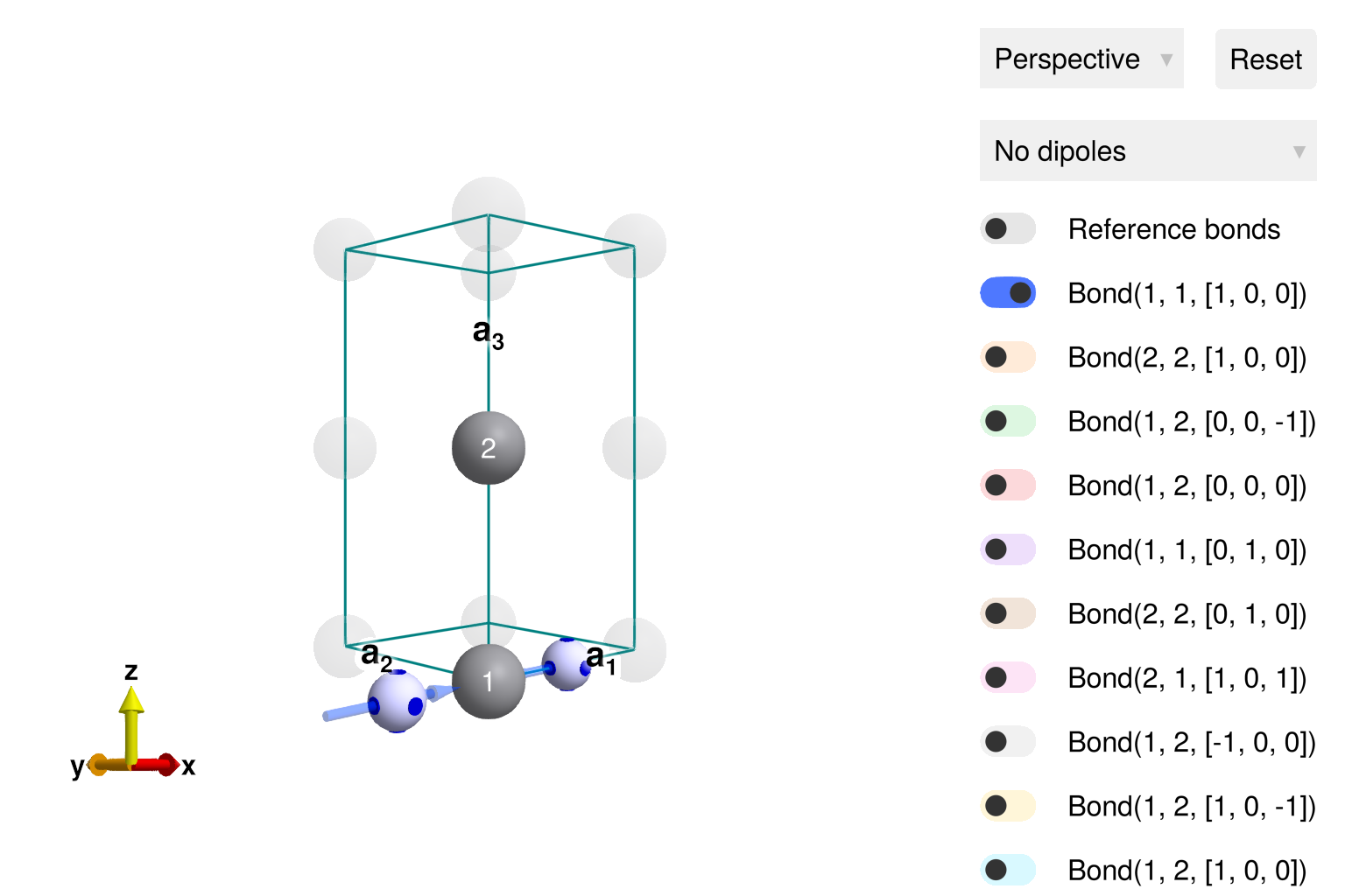

Energy minimization yields a Néel order with canting

randomize_spins!(sys)
minimize_energy!(sys)
plot_spins(sys)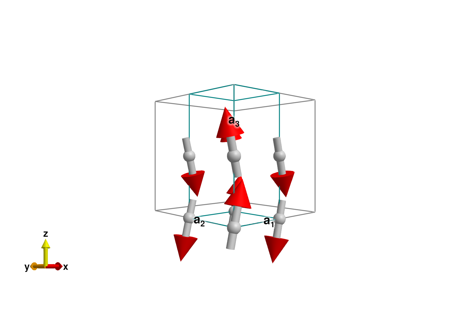

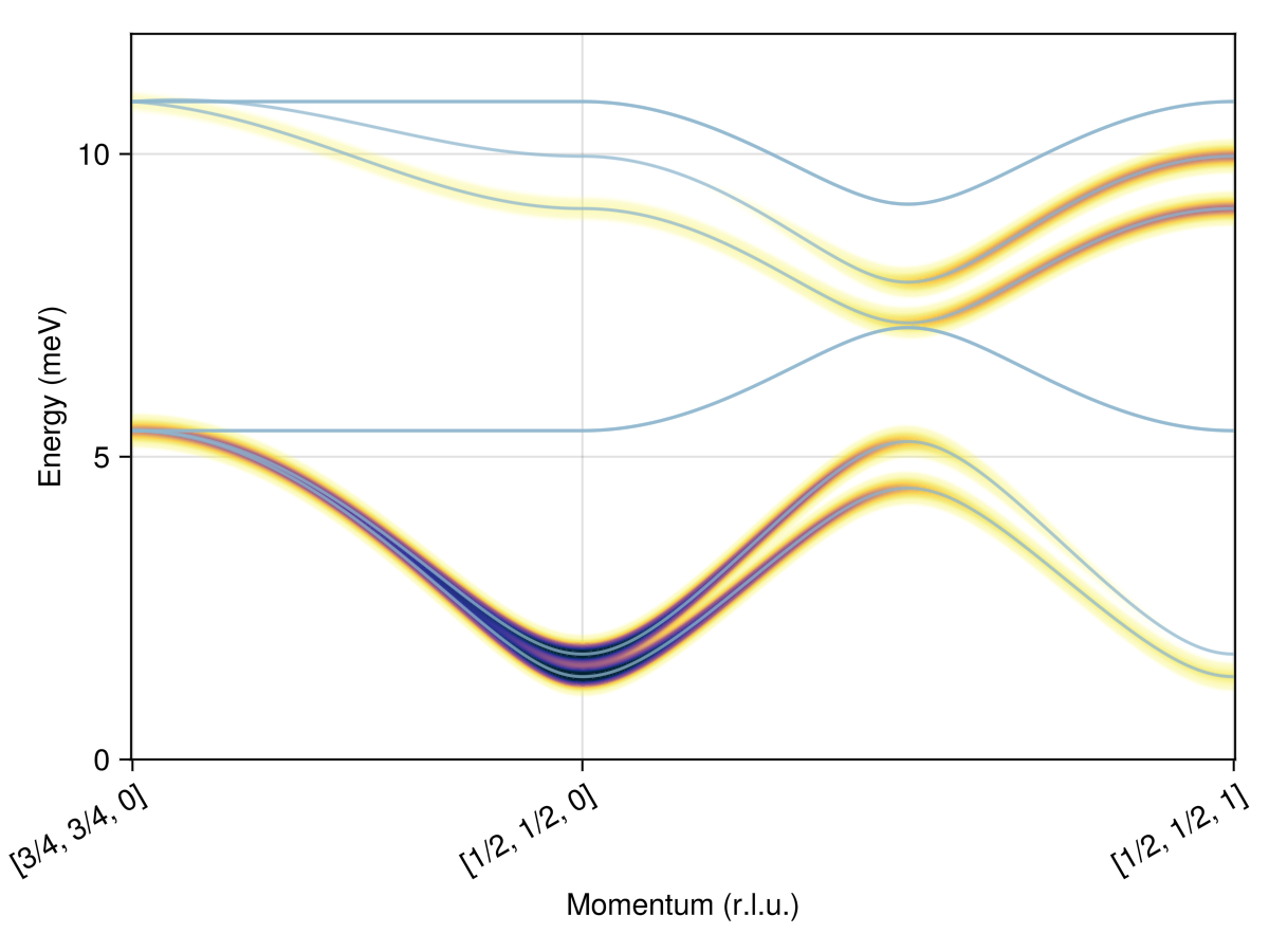
Plot the spin wave spectrum along a path

swt = SpinWaveTheory(sys; measure=ssf_perp(sys))
qs = [[0.75, 0.75, 0], [0.5, 0.5, 0], [0.5, 0.5, 1]]
path = q_space_path(cryst, qs, 400)
res = intensities_bands(swt, path)
plot_intensities(res; units)