Download this example as Julia file or Jupyter notebook.
SW12 - Triangular lattice with easy plane
This is a Sunny port of SpinW Tutorial 12, originally authored by Sandor Toth. It calculates the spin wave dispersion of a triangular lattice model with antiferromagnetic interactions and easy-plane single-ion anisotropy.
Load packages
using Sunny, GLMakieBuild a triangular lattice with arbitrary lattice constant of 3 Å.
latvecs = lattice_vectors(3, 3, 4, 90, 90, 120)
cryst = Crystal(latvecs, [[0, 0, 0]])
Crystal
Spacegroup 'P 6/m m m' (191)
Lattice params a=3, b=3, c=4, α=90°, β=90°, γ=120°
Cell volume 31.18
Wyckoff 1a (site sym. '6/mmm'):
1. [0, 0, 0]
Build a system with exchange +1 meV along nearest neighbor bonds. Set the lattice size in anticipation of a magnetic ordering with 3×3 cells.
s = 3/2
J1 = +1.0
sys = System(cryst, [1 => Moment(; s, g=2)], :dipole; dims=(3, 3, 1))
set_exchange!(sys, J1, Bond(1, 1, [1, 0, 0]))
Set an easy-axis anisotropy operator $+D S_z^2$ using set_onsite_coupling!. Important note: When introducing a single-ion anisotropy in :dipole mode, Sunny will automatically include a classical-to-quantum correction factor, as described in the document Interaction Renormalization. For an anisotropy operator that is quadratic in the spin operators, Sunny will automatically renormalize the interaction strength as $D → (1 - 1/2s) D$. We must "undo" Sunny's classical-to-quantum rescaling factor to reproduce the SpinW calculation. Alternatively, renormalization can be disabled by selecting the system mode :dipole_uncorrected instead of :dipole.
undo_classical_to_quantum_rescaling = 1 / (1 - 1/2s)
D = 0.2 * undo_classical_to_quantum_rescaling
set_onsite_coupling!(sys, S -> D*S[3]^2, 1)
randomize_spins!(sys)
minimize_energy!(sys)
plot_spins(sys; ndims=2)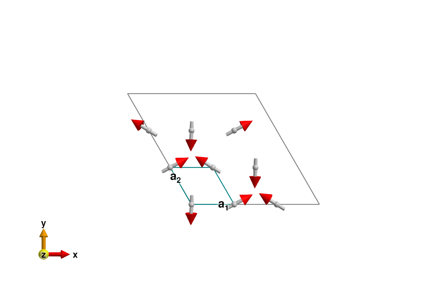
Plot the spin wave spectrum for a path through $𝐪$-space.
qs = [[0, 0, 0], [1, 1, 0]]
path = q_space_path(cryst, qs, 400)
swt = SpinWaveTheory(sys; measure=ssf_perp(sys))
res = intensities_bands(swt, path)
plot_intensities(res)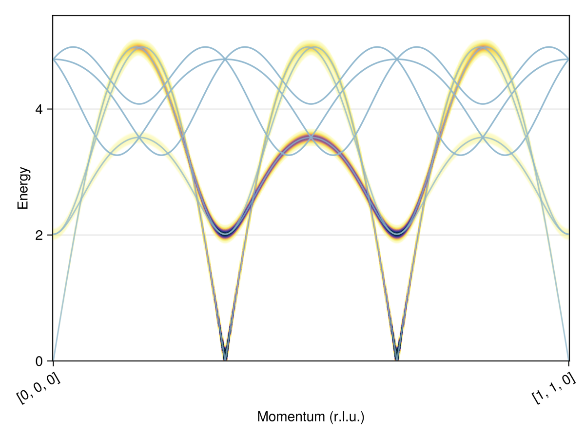
To select a specific linear combination of spin structure factor (SSF) components in global Cartesian coordinates, one can use ssf_custom. Here we calculate and plot the real part of $\mathcal{S}^{zz}(𝐪, ω)$.
measure = ssf_custom(sys) do q, ssf
    return real(ssf[3, 3])
end
swt = SpinWaveTheory(sys; measure)
res = intensities_bands(swt, path)
plot_intensities(res)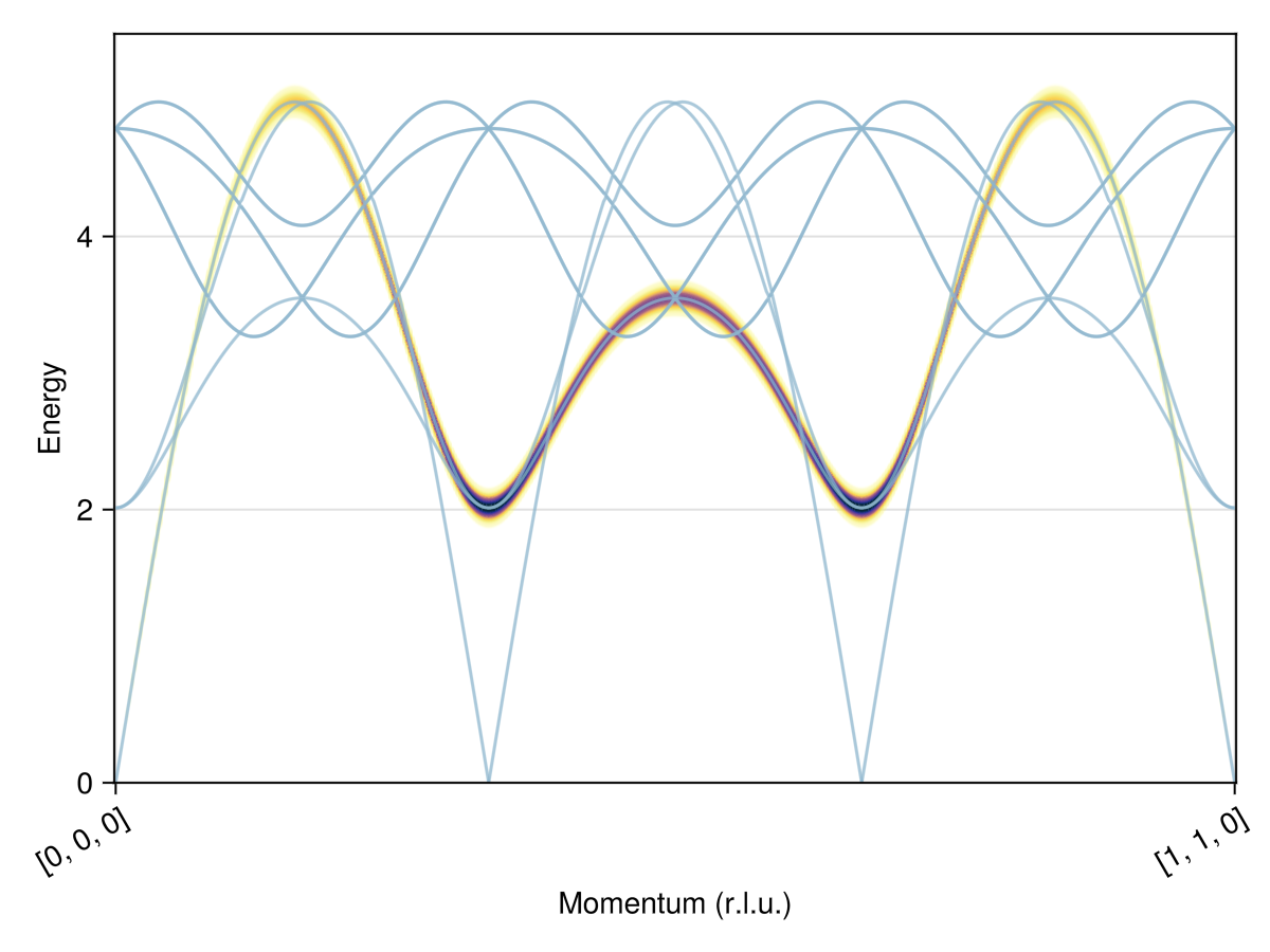
It's also possible to get data for the full 3×3 SSF. For example, this is the SSF for the 7th energy band, at the 10th $𝐪$-point along the path.
measure = ssf_custom((q, ssf) -> ssf, sys)
swt = SpinWaveTheory(sys; measure)
res = intensities_bands(swt, path)
res.data[7, 10]
3×3 StaticArraysCore.SMatrix{3, 3, ComplexF64, 9} with indices SOneTo(3)×SOneTo(3):
0.241929+0.0im … 1.11514e-14+1.60472e-13im
3.2363e-13-0.241929im 1.60472e-13-1.11514e-14im
1.11514e-14-1.60472e-13im 1.06956e-25+0.0im