Download this example as Julia file or Jupyter notebook.
3. Multi-flavor spin wave simulations of FeI₂
This tutorial illustrates various advanced features such as symmetry analysis, energy minimization, and spin wave theory with multi-flavor bosons.
Our context will be FeI₂, an effective spin-1 material with strong single-ion anisotropy. Quadrupolar fluctuations give rise to a single-ion bound state that is observable in neutron scattering, and cannot be described by a dipole-only model. We will use the linear spin wave theory of SU(3) coherent states (i.e. 2-flavor bosons) to model the magnetic spectrum of FeI₂. The original study was performed in Bai et al., Nat. Phys. 17, 467–472 (2021).
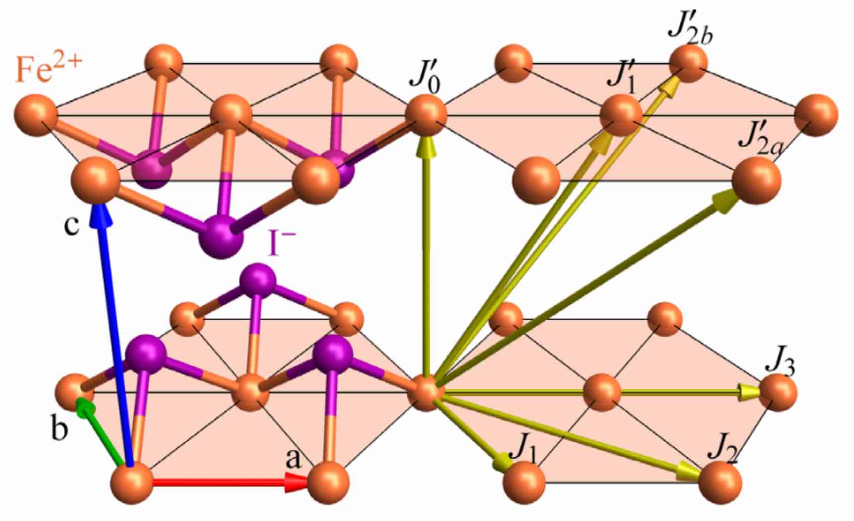
The Fe atoms are arranged in stacked triangular layers. The effective spin Hamiltonian takes the form,
\[\mathcal{H}=\sum_{(i,j)} 𝐒_i ⋅ J_{ij} 𝐒_j - D\sum_i \left(S_i^z\right)^2,\]
where the exchange matrices $J_{ij}$ between bonded sites $(i,j)$ include competing ferromagnetic and antiferromagnetic interactions. This model also includes a strong easy axis anisotropy, $D > 0$.
Load packages.
using Sunny, GLMakieConstruct the chemical cell of FeI₂ by specifying the lattice vectors and the full set of atoms.
units = Units(:meV, :angstrom)
a = b = 4.05012  # Lattice constants for triangular lattice (Å)
c = 6.75214      # Spacing between layers (Å)
latvecs = lattice_vectors(a, b, c, 90, 90, 120)
positions = [[0, 0, 0], [1/3, 2/3, 1/4], [2/3, 1/3, 3/4]]
types = ["Fe", "I", "I"]
cryst = Crystal(latvecs, positions; types)
Crystal
Spacegroup 'P -3 m 1' (164)
Lattice params a=4.05, b=4.05, c=6.752, α=90°, β=90°, γ=120°
Cell volume 95.92
Type 'Fe', Wyckoff 1a (site sym. '-3m.'):
1. [0, 0, 0]
Type 'I', Wyckoff 2d (site sym. '3m.'):
2. [1/3, 2/3, 1/4]
3. [2/3, 1/3, 3/4]
Observe that the space group 'P -3 m 1' (164) has been inferred, as well as point group symmetries. Only the Fe atoms are magnetic, so we focus on them with subcrystal. Importantly, the new crystal retains the symmetry information for spacegroup 164.
cryst = subcrystal(cryst, "Fe")
view_crystal(cryst)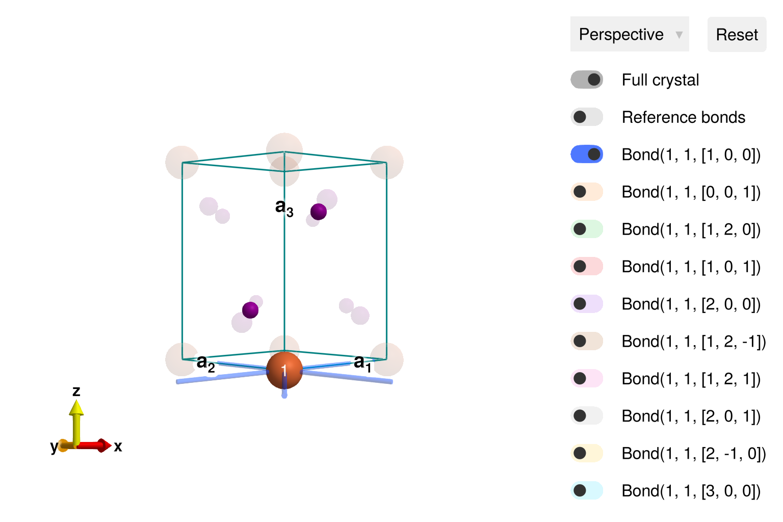
Symmetry analysis
The command print_symmetry_table provides a list of all the symmetry-allowed interactions out to 8 Å.
print_symmetry_table(cryst, 8.0)Atom 1
Type 'Fe', position [0, 0, 0], Wyckoff 1a
Allowed g-tensor: [A 0 0
0 A 0
0 0 B]
Allowed anisotropy in Stevens operators:
c₁*𝒪[2,0] +
c₂*𝒪[4,-3] + c₃*𝒪[4,0] +
c₄*𝒪[6,-3] + c₅*𝒪[6,0] + c₆*𝒪[6,6]
Bond(1, 1, [1, 0, 0])
Distance 4.050120000, coordination 6
Connects 'Fe' at [0, 0, 0] to 'Fe' at [1, 0, 0]
Allowed exchange matrix: [A 0 0
0 B D
0 D C]
Bond(1, 1, [0, 0, 1])
Distance 6.752140000, coordination 2
Connects 'Fe' at [0, 0, 0] to 'Fe' at [0, 0, 1]
Allowed exchange matrix: [A 0 0
0 A 0
0 0 B]
Bond(1, 1, [1, 2, 0])
Distance 7.015013617, coordination 6
Connects 'Fe' at [0, 0, 0] to 'Fe' at [1, 2, 0]
Allowed exchange matrix: [A 0 0
0 B D
0 D C]
Bond(1, 1, [1, 0, 1])
Distance 7.873681896, coordination 12
Connects 'Fe' at [0, 0, 0] to 'Fe' at [1, 0, 1]
Allowed exchange matrix: [A F E
F B D
E D C]The allowed $g$-tensor is expressed as a 3×3 matrix in the free coefficients A, B, ... The allowed single-ion anisotropy is expressed as a linear combination of Stevens operators. The latter correspond to polynomials of the spin operators, as we will describe below.
The allowed exchange interactions are given as 3×3 matrices for representative bonds. The notation Bond(i, j, n) indicates a bond between atom indices i and j, with cell offset n. Note that the order of the pair $(i, j)$ is significant if the exchange tensor contains antisymmetric Dzyaloshinskii–Moriya (DM) interactions.
The bonds can be visualized in the view_crystal interface. By default, Bond(1, 1, [1,0,0]) is toggled on, to show the 6 nearest-neighbor Fe-Fe bonds on a triangular lattice layer. Toggling Bond(1, 1, [0,0,1]) shows the Fe-Fe bond between layers, etc.
Defining the spin model
Construct a System with spin $s=1$ and $g=2$ for the Fe ions.
Recall that quantum spin-1 is, in reality, a linear combination of basis states $|m⟩$ with well-defined angular momentum $m = -1, 0, 1$. FeI₂ has a strong easy-axis anisotropy, which stabilizes a single-ion bound state of zero angular momentum, $|m=0⟩$. Such a bound state is inaccessible to traditional spin wave theory, which works with dipole expectation values of fixed magnitude. This physics is, however, well captured with a theory of SU(N) coherent states, where $N = 2S+1 = 3$ is the number of levels. Activate this generalized theory by selecting :SUN mode instead of :dipole mode.
An optional seed for random number generation can be used to to make the calculation exactly reproducible.
sys = System(cryst, [1 => Moment(s=1, g=2)], :SUN; seed=2)System [SU(3)]
Supercell (1×1×1)×1
Energy per site 0
Set the exchange interactions for FeI₂ following the fits of Bai et al.
J1pm   = -0.236 # (meV)
J1pmpm = -0.161
J1zpm  = -0.261
J2pm   = 0.026
J3pm   = 0.166
J′0pm  = 0.037
J′1pm  = 0.013
J′2apm = 0.068

J1zz   = -0.236
J2zz   = 0.113
J3zz   = 0.211
J′0zz  = -0.036
J′1zz  = 0.051
J′2azz = 0.073

J1xx = J1pm + J1pmpm
J1yy = J1pm - J1pmpm
J1yz = J1zpm

set_exchange!(sys, [J1xx   0.0    0.0;
                    0.0    J1yy   J1yz;
                    0.0    J1yz   J1zz], Bond(1,1,[1,0,0]))
set_exchange!(sys, [J2pm   0.0    0.0;
                    0.0    J2pm   0.0;
                    0.0    0.0    J2zz], Bond(1,1,[1,2,0]))
set_exchange!(sys, [J3pm   0.0    0.0;
                    0.0    J3pm   0.0;
                    0.0    0.0    J3zz], Bond(1,1,[2,0,0]))
set_exchange!(sys, [J′0pm  0.0    0.0;
                    0.0    J′0pm  0.0;
                    0.0    0.0    J′0zz], Bond(1,1,[0,0,1]))
set_exchange!(sys, [J′1pm  0.0    0.0;
                    0.0    J′1pm  0.0;
                    0.0    0.0    J′1zz], Bond(1,1,[1,0,1]))
set_exchange!(sys, [J′2apm 0.0    0.0;
                    0.0    J′2apm 0.0;
                    0.0    0.0    J′2azz], Bond(1,1,[1,2,1]))
The function set_onsite_coupling! assigns a single-ion anisotropy. The argument can be constructed using spin_matrices or stevens_matrices. Here we use Julia's anonymous function syntax to assign an easy-axis anisotropy along the direction $\hat{z}$.
D = 2.165 # (meV)
set_onsite_coupling!(sys, S -> -D*S[3]^2, 1)
Finding the ground state
The model parameters have already been fitted so that energy minimization yields the physically correct ground state. Knowing this, one could manually set the magnetic configuration by calling set_dipole! at each site. Alternatively, Sunny provides tools to interactively search for the ground state.
Use resize_supercell to create a relatively large system of 4×4×4 chemical cells. Call randomize_spins! and minimize_energy! in sequence.
sys = resize_supercell(sys, (4, 4, 4))
randomize_spins!(sys)
minimize_energy!(sys)
Converged in 53 iterationsDespite successful convergence to a local energy minimum, defects in the spin configuration are visually apparent.
plot_spins(sys; color=[S[3] for S in sys.dipoles])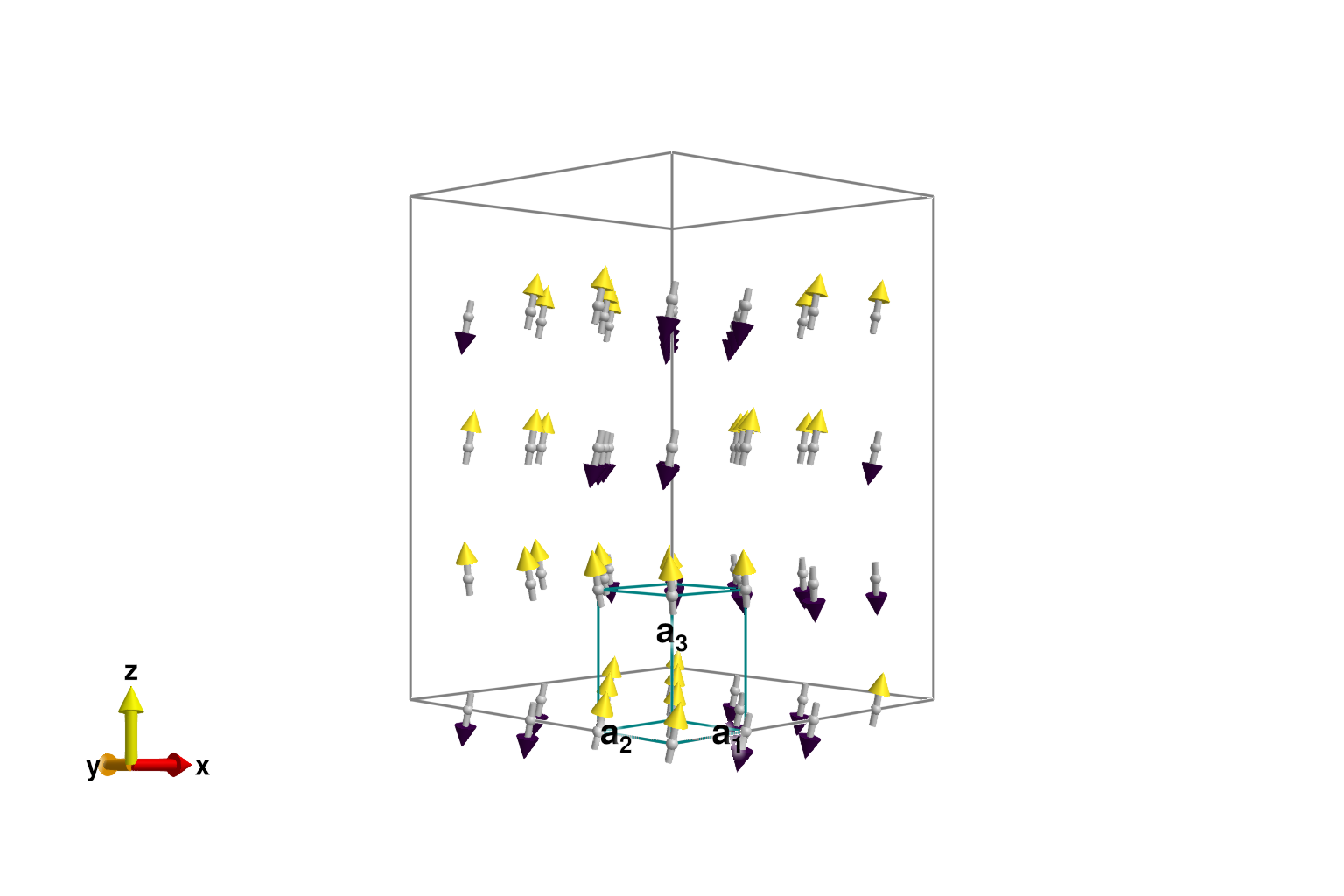
Finding the true ground state can be a challenging task. If the system is not too large, a good strategy is repeated randomization and then energy minimization. This particular system might require about 30 minimization runs to find the defect-free ground state.
Another tool is print_wrapped_intensities. It reports weights analogous to the static structure factor $\mathcal{S}(𝐪)$, but without accounting for phase interference between magnetic sublattices. To calculate the true $\mathcal{S}(𝐪)$, use instead SampledCorrelationsStatic.
print_wrapped_intensities(sys)Dominant wavevectors for spin sublattices:
[-1/4, 1/4, 1/4] 28.40% weight
[1/4, -1/4, -1/4] 28.40%
[1/4, 0, 1/4] 3.21%
[-1/4, 0, -1/4] 3.21%
[1/4, 0, 0] 3.12%
[-1/4, 0, 0] 3.12%
[1/4, 0, 1/2] 3.11%
[-1/4, 0, 1/2] 3.11%
[-1/4, 0, 1/4] 3.04%
[1/4, 0, -1/4] 3.04%
[-1/4, 1/4, 0] 3.04%
... ...The correct ground state for FeI₂ is known to be a generalized spiral with one of three propagation wavevectors, $[0, -1/4, 1/4]$ or $[1/4, 0, 1/4]$ or $[-1/4, 1/4, 1/4]$, which are equivalent under 120° rotations. The result of print_wrapped_intensities hints at this spiral phase.
Let's break the 3-fold symmetry by hand. The function suggest_magnetic_supercell takes any number of propagation wavevectors and suggests a commensurate magnetic cell.
suggest_magnetic_supercell([[0, -1/4, 1/4]])Possible magnetic supercell in multiples of lattice vectors:
[1 0 0; 0 1 -2; 0 1 2]
for the rationalized wavevectors:
[[0, -1/4, 1/4]]After calling reshape_supercell, it becomes easy to find the ground state. Plot the system again, now including "ghost" spins out to 12Å. The correct two-up, two-down magnetic order is visually apparent.
sys_min = reshape_supercell(sys, [1 0 0; 0 1 -2; 0 1 2])
randomize_spins!(sys_min)
minimize_energy!(sys_min)
plot_spins(sys_min; color=[S[3] for S in sys_min.dipoles], ghost_radius=12)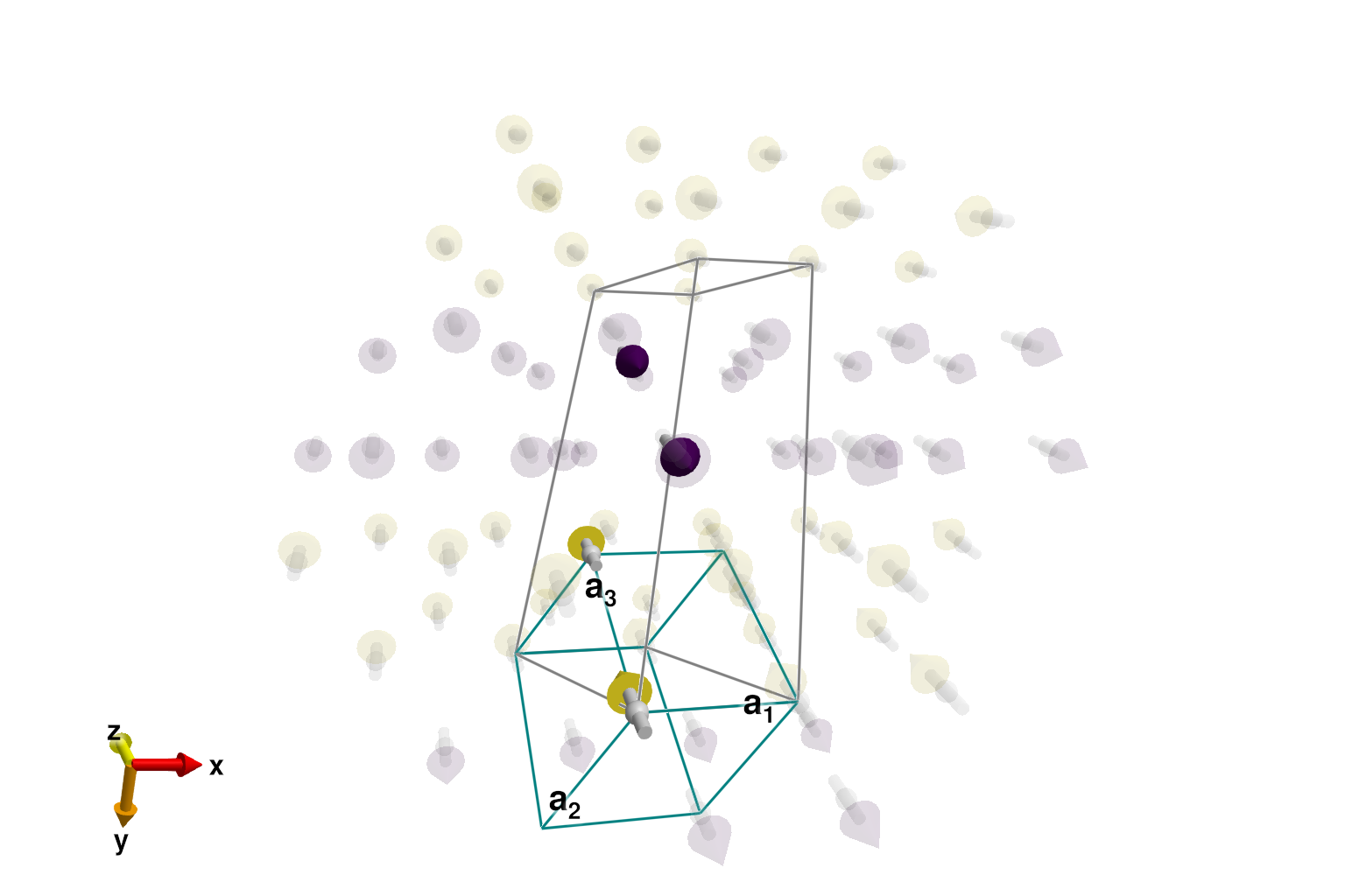
Spin wave theory
Now that the system has been relaxed to an energy minimized ground state, we can calculate the spin wave spectrum. Because the system was constructed in :SUN mode, the spin wave calculation will automatically employ bosons with `N = 2s+1 = 3 flavors.
swt = SpinWaveTheory(sys_min; measure=ssf_perp(sys_min))SpinWaveTheory [SU(3)]
4 atoms
Calculate and plot the spectrum along a momentum-space path that connects a sequence of high-symmetry $𝐪$-points. This interface abstracts over the underlying calculator type.
qs = [[0,0,0], [1,0,0], [0,1,0], [1/2,0,0], [0,1,0], [0,0,0]]
path = q_space_path(cryst, qs, 500)
res = intensities_bands(swt, path)
plot_intensities(res; units, ylims=(0, 10), title="Single Crystal Bands")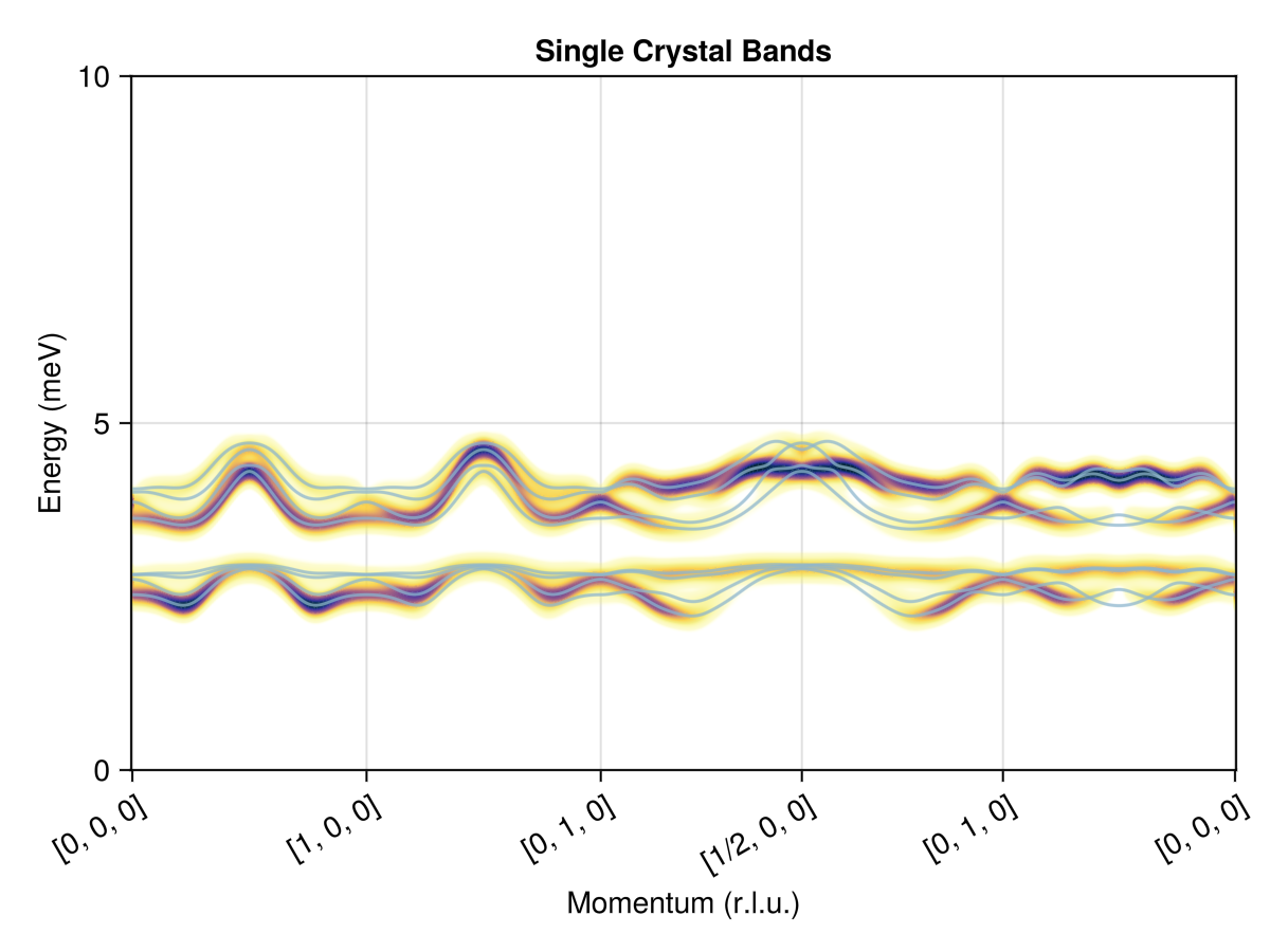
To make direct comparison with inelastic neutron scattering (INS) data, we must account for empirical broadening of the data. Model this using a lorentzian kernel, with a full-width at half-maximum of 0.3 meV.
kernel = lorentzian(fwhm=0.3)
energies = range(0, 10, 300);  # 0 < ω < 10 (meV)
Also, a real FeI₂ sample will exhibit competing magnetic domains. We use domain_average to average over the three possible domain orientations. This involves 120° rotations about the axis $\hat{z} = [0, 0, 1]$ in global Cartesian coordinates.
rotations = [([0,0,1], n*(2π/3)) for n in 0:2]
weights = [1, 1, 1]
res = domain_average(cryst, path; rotations, weights) do path_rotated
    intensities(swt, path_rotated; energies, kernel)
end
plot_intensities(res; units, colormap=:viridis, title="Domain Averaged Intensities")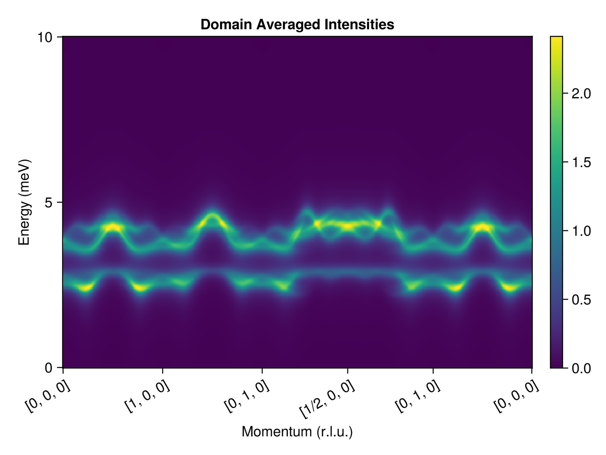
This result can be directly compared to experimental neutron scattering data from Bai et al.
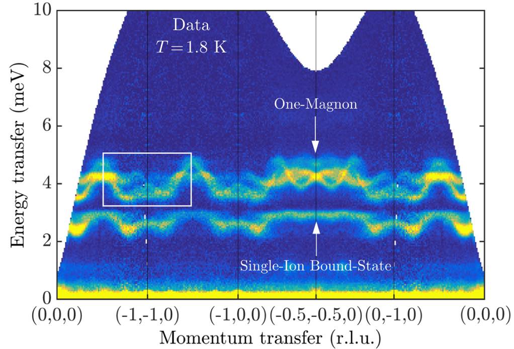
(The publication figure used a non-standard coordinate system to label the wave vectors.)
To get this agreement, the theory of SU(3) coherent states is essential. The lower band has large quadrupolar character and arises from the strong easy-axis anisotropy of FeI₂.
An interesting exercise is to repeat the same study, but using :dipole mode instead of :SUN. That alternative choice would constrain the coherent state dynamics to the space of dipoles only, and the flat band of single-ion bound states would be missing.