Download this example as Julia file or Jupyter notebook.

6. Dynamical quench into CP² skyrmion liquid

This example demonstrates a non-equilibrium study of SU(3) spin dynamics leading to the formation of a CP² skyrmion liquid. As proposed in Zhang et al., Nature Communications 14, 3626 (2023), CP² skyrmions are topological defects that involve both the dipolar and quadrupolar parts of quantum spin-1, and can be studied using the formalism SU(3) coherent states.

This study uses the SU(N) generalization of Landau-Lifshitz spin dynamics, with Langevin coupling to a thermal bath, as described in Dahlbom et al., Phys. Rev. B 106, 235154 (2022). Beginning from an initial high-temperature state, the dynamics following a rapid quench in temperature gives rise a disordered liquid of CP² skyrmions.

using Sunny, GLMakie

Begin with a Crystal cell for the triangular lattice.

lat_vecs = lattice_vectors(1, 1, 10, 90, 90, 120)
positions = [[0, 0, 0]]
cryst = Crystal(lat_vecs, positions)

Crystal
Spacegroup 'P 6/m m m' (191)
Lattice params a=1, b=1, c=10, α=90°, β=90°, γ=120°
Cell volume 8.66
Wyckoff 1a (point group '6/mmm'):
   1. [0, 0, 0]

Create a spin System containing $L×L$ cells. Following previous worse, select $g=-1$ so that the Zeeman coupling has the form $-𝐁⋅𝐬$.

L = 40
sys = System(cryst, [1 => Moment(s=1, g=-1)], :SUN; dims=(L, L, 1))

System [SU(3)]
Supercell (40×40×1)×1
Energy per site 0

The Hamiltonian,

\[\mathcal{H} = \sum_{\langle i,j \rangle} J_{ij}( \hat{S}_i^x \hat{S}_j^x + \hat{S}_i^y \hat{S}_j^y + \Delta\hat{S}_i^z \hat{S}_j^z) - h\sum_{i}\hat{S}_i^z + D\sum_{i}(\hat{S}_i^z)^2,\]

contains competing ferromagnetic first-neighbor and antiferromagnetic second-neighbor exchange terms on a triangular lattice. Both exchange matrices include anisotropy in the $\hat{z}$ direction. Additionally, there is an external magnetic field $h$ and an easy-plane single-ion anisotropy $D$. Select parameters for a point in the Zhang et al. phase diagram where the CP² skyrmions are stable.

J1 = -1           # Nearest-neighbor ferromagnetic
J2 = (2.0/(1+√5)) # Tune competing exchange to set skyrmion scale length
Δ = 2.6           # Exchange anisotropy

ex1 = J1 * [1 0 0;
            0 1 0;
            0 0 Δ]
ex2 = J2 * [1 0 0;
            0 1 0;
            0 0 Δ]
set_exchange!(sys, ex1, Bond(1, 1, [1, 0, 0]))
set_exchange!(sys, ex2, Bond(1, 1, [1, 2, 0]))

h = 15.5         # External field in energy units
field = set_field!(sys, [0, 0, h])

D = 19.0         # Easy-plane anisotropy
set_onsite_coupling!(sys, S -> D*S[3]^2, 1)

Initialize system to an infinite temperature (fully randomized) initial condition.

We will study a temperature quench process using a generalized Langevin spin dynamics. In this SU(3) treatment of quantum spin-1, the dynamics include coupled dipoles and quadrupoles. Select a relatively small damping magnitude to overcome local minima, and disable thermal fluctuations.

damping = 0.05
kT = 0;

The first step is to estimate a reasonable integration timestep dt. In this case, a random spin configuration gives a tighter bound than does an energy-minimized configuration. A relatively large error tolerance is OK for this phenomenological study.

randomize_spins!(sys)
integrator = Langevin(; damping, kT)
suggest_timestep(sys, integrator; tol=0.05)

Consider dt ≈ 0.01104 for this spin configuration at tol = 0.05.

Apply the suggested timestep.

integrator.dt = 0.01;

Now run the dynamical quench starting from a randomized configuration. The field frames stores the system spin configuration, as SU(3) coherent states, at three different times during the quenching process.

randomize_spins!(sys)
τs = [4, 16, 256]   # Times to record snapshots
frames = []         # Empty array to store snapshots
for i in eachindex(τs)
    dur = i == 1 ? τs[1] : τs[i] - τs[i-1] # Determine the length of time to simulate
    numsteps = round(Int, dur/integrator.dt)
    for _ in 1:numsteps                    # Perform the integration
        step!(sys, integrator)
    end
    push!(frames, copy(sys.coherents))     # Save a snapshot spin configuration
end

Visualize the state of the system contained in each snapshot by plotting the SU(3) Berry phase curvature over triangular plaquettes. This is a measure of CP² skyrmion density. The function plot_triangular_plaquettes is not part of the core Sunny package, but rather something you could define yourself using Makie. Find this helper function at examples/extra/Plotting/.

include(pkgdir(Sunny, "examples", "extra", "Plotting", "plotting2d.jl"))

function sun_berry_curvature(z₁, z₂, z₃)
    z₁, z₂, z₃ = normalize.((z₁, z₂, z₃))
    n₁ = z₁ ⋅ z₂
    n₂ = z₂ ⋅ z₃
    n₃ = z₃ ⋅ z₁
    return angle(n₁ * n₂ * n₃)
end

plot_triangular_plaquettes(sun_berry_curvature, frames; size=(600, 200),
    offset_spacing=10, texts=["\tt = "*string(τ) for τ in τs], text_offset=(0, 6)
)

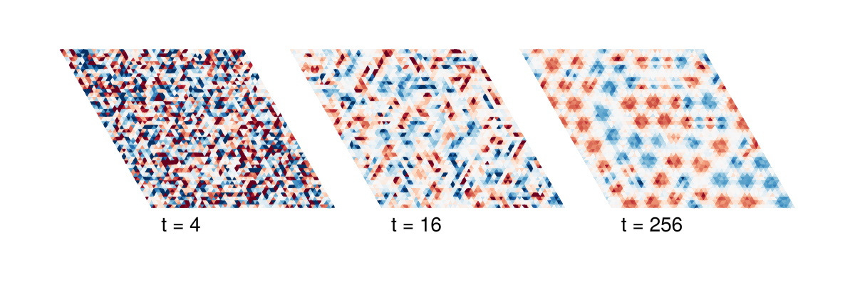
The times are given in $\hbar/|J_1|$. The white background corresponds to a quantum paramagnetic state, where the local spin exhibits a strong quadrupole moment and little or no dipole moment. At late times, there are well-formed skyrmions of positive (red) and negative (blue) charge, and various metastable spin configurations. A full-sized version of this figure is available in Dahlbom et al..