Download this example as Julia file or Jupyter notebook.
SW15 - Ba₃NbFe₃Si₂O₁₄
This is a Sunny port of SpinW Tutorial 15, originally authored by Sandor Toth. It calculates the linear spin wave theory spectrum of Ba₃NbFe₃Si₂O₁₄. The ground state is an incommensurate spiral, which can be directly studied using the functions minimize_spiral_energy! and SpinWaveTheorySpiral.
Load packages
using Sunny, GLMakieSpecify the Ba₃NbFe₃Si₂O₁₄ Crystal cell following Marty et al., Phys. Rev. Lett. 101, 247201 (2008).
units = Units(:meV, :angstrom)
a = b = 8.539 # (Å)
c = 5.2414
latvecs = lattice_vectors(a, b, c, 90, 90, 120)
types = ["Fe", "Nb", "Ba", "Si", "O", "O", "O"]
positions = [[0.24964,0,0.5], [0,0,0], [0.56598,0,0], [2/3,1/3,0.5220],
             [2/3,1/3,0.2162], [0.5259,0.7024,0.3536], [0.7840,0.9002,0.7760]]
langasite = Crystal(latvecs, positions, 150; types)
cryst = subcrystal(langasite, "Fe")
view_crystal(cryst)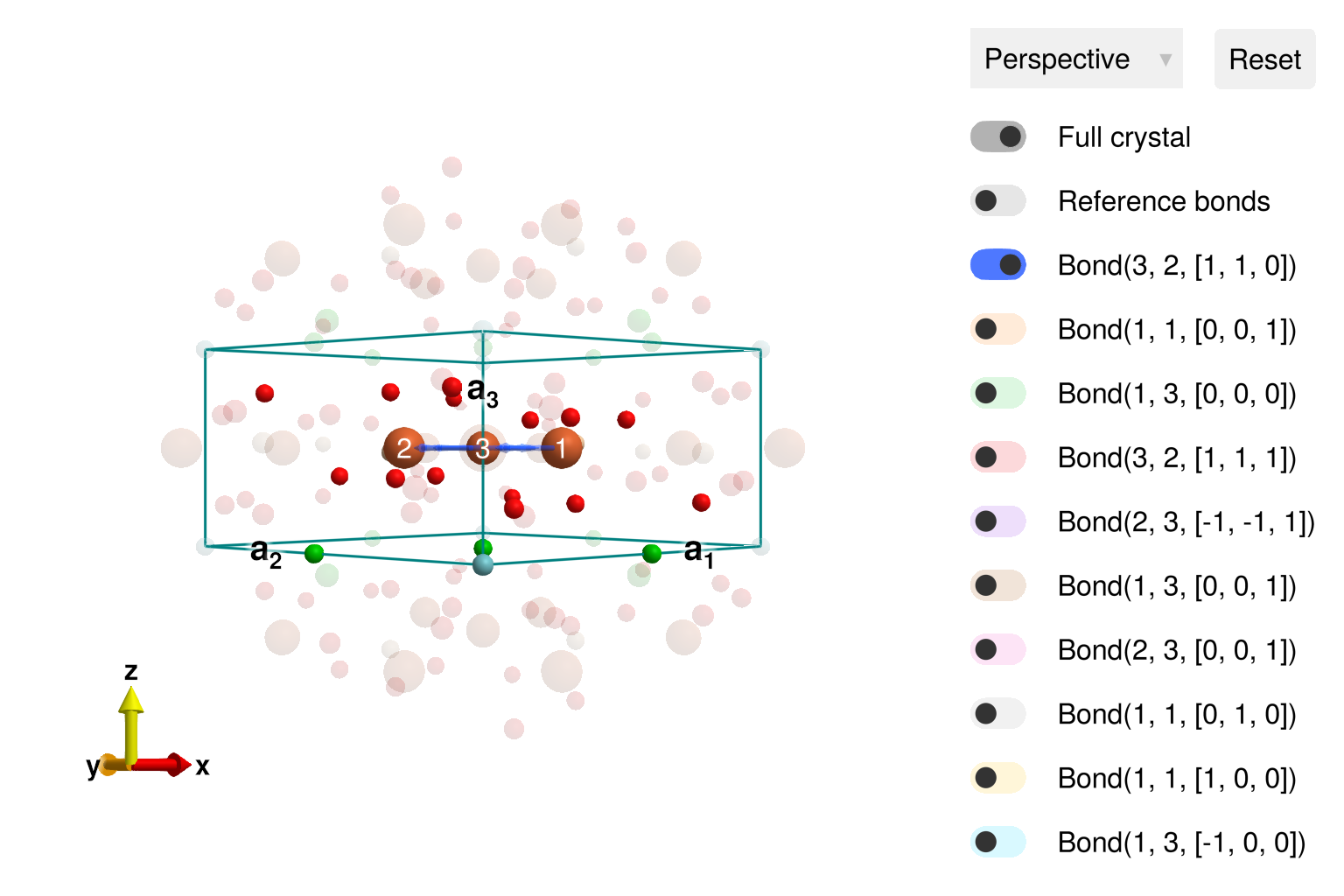
Create a System and set exchange interactions as parametrized in Loire et al., Phys. Rev. Lett. 106, 207201 (2011).
sys = System(cryst, [1 => Moment(s=5/2, g=2)], :dipole)
J₁ = 0.85
J₂ = 0.24
J₃ = 0.053
J₄ = 0.017
J₅ = 0.24
set_exchange!(sys, J₁, Bond(3, 2, [1,1,0]))
set_exchange!(sys, J₄, Bond(1, 1, [0,0,1]))
set_exchange!(sys, J₂, Bond(1, 3, [0,0,0]))
The final two exchanges are set according to the desired chirality $ϵ_T$ of the magnetic structure.
ϵT = -1
if ϵT == -1
    set_exchange!(sys, J₃, Bond(2, 3, [-1,-1,1]))
    set_exchange!(sys, J₅, Bond(3, 2, [1,1,1]))
elseif ϵT == 1
    set_exchange!(sys, J₅, Bond(2, 3, [-1,-1,1]))
    set_exchange!(sys, J₃, Bond(3, 2, [1,1,1]))
else
    error("Chirality must be ±1")
end
This compound is known to have a spiral order with approximate propagation wavevector $𝐤 ≈ [0, 0, 1/7]$. Search for this magnetic order with minimize_spiral_energy!. Due to reflection symmetry, one of two possible propagation wavevectors may appear, $𝐤 = ± [0, 0, 0.1426…]$. Note that $k_z = 0.1426…$ is very close to $1/7 = 0.1428…$.
axis = [0, 0, 1]
randomize_spins!(sys)
k = minimize_spiral_energy!(sys, axis)
3-element StaticArraysCore.SVector{3, Float64} with indices SOneTo(3):
-2.7156918884886985e-12
3.1620796348965177e-12
0.1426460465616074We can visualize the full magnetic cell using repeat_periodically_as_spiral, which includes 7 rotated copies of the chemical cell.
sys_enlarged = repeat_periodically_as_spiral(sys, (1, 1, 7); k, axis)
plot_spins(sys_enlarged; color=[S[1] for S in sys_enlarged.dipoles])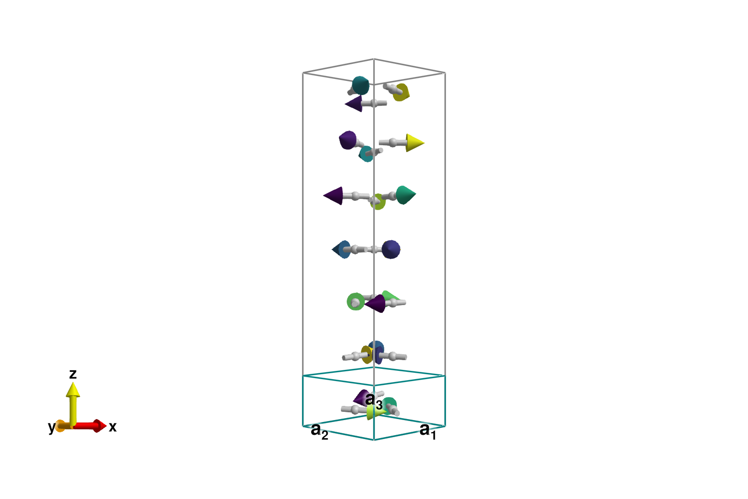
One could perform a spin wave calculation using either SpinWaveTheory on sys_enlarged, or SpinWaveTheorySpiral on the original sys. The latter has some restrictions on the interactions, but allows for our slightly incommensurate wavevector $𝐤$.
measure = ssf_perp(sys)
swt = SpinWaveTheorySpiral(sys; measure, k, axis)
SpinWaveTheorySpiral(SpinWaveTheory(System([Dipole mode], Supercell (1×1×1)×3, Energy per site 9.601), Sunny.SWTDataDipole(StaticArraysCore.SMatrix{3, 3, Float64, 9}[[0.9189241784494253 -0.3189955390709207 0.23199181087681034; -0.2191621224123797 0.07607998694533824 0.9727177389593028; -0.327942553446103 -0.9446976667904129 1.1732376753802308e-10], [0.5621068037460668 0.3954434752276905 0.726402367205826; 0.5941128060303403 0.4179597741326105 -0.6872696711755673; -0.5753832765149991 0.8178839068638434 3.8197062349963546e-11], [-0.003004595304993391 -0.28543225432580327 -0.9583941780903843; 0.010087952288498904 0.9583410842785403 -0.28544806778546744; 0.9999446012783298 -0.010525890666438649 -1.5916817291607023e-10]], StaticArraysCore.SVector{3, Float64}[[1.8378483568988502, -0.6379910781418413, 0.4639836217536208] [1.1242136074921334, 0.7908869504553809, 1.452804734411652] [-0.006009190609986776, -0.570864508651606, -1.916788356180767]; [-0.43832424482475896, 0.15215997389067634, 1.9454354779186047] [1.18822561206068, 0.8359195482652204, -1.3745393423511338] [0.020175904576997798, 1.9166821685570794, -0.5708961355709347]; [-0.6558851068922059, -1.8893953335808253, 2.346475350760461e-10] [-1.150766553029998, 1.6357678137276863, 7.639412469992708e-11] [1.9998892025566588, -0.021051781332877287, -3.183363458321403e-10]], Sunny.StevensExpansion[Sunny.StevensExpansion([0.0], [0.0, 0.0, 0.0, 0.0, 0.0], [0.0, 0.0, 0.0, 0.0, 0.0, 0.0, 0.0, 0.0, 0.0], [0.0, 0.0, 0.0, 0.0, 0.0, 0.0, 0.0, 0.0, 0.0, 0.0, 0.0, 0.0, 0.0], 0), Sunny.StevensExpansion([0.0], [0.0, 0.0, 0.0, 0.0, 0.0], [0.0, 0.0, 0.0, 0.0, 0.0, 0.0, 0.0, 0.0, 0.0], [0.0, 0.0, 0.0, 0.0, 0.0, 0.0, 0.0, 0.0, 0.0, 0.0, 0.0, 0.0, 0.0], 0), Sunny.StevensExpansion([0.0], [0.0, 0.0, 0.0, 0.0, 0.0], [0.0, 0.0, 0.0, 0.0, 0.0, 0.0, 0.0, 0.0, 0.0], [0.0, 0.0, 0.0, 0.0, 0.0, 0.0, 0.0, 0.0, 0.0, 0.0, 0.0, 0.0, 0.0], 0)], [1.5811388300841898, 1.5811388300841898, 1.5811388300841898]), MeasureSpec, 1.0e-8), [-2.7156918884886985e-12, 3.1620796348965177e-12, 0.1426460465616074], 3, [0.0, 0.0, 1.0], Matrix{StaticArraysCore.SMatrix{3, 3, ComplexF64, 9}}[[[0.0 + 0.0im 0.0 + 0.0im 0.0 + 0.0im; 0.0 + 0.0im 0.0 + 0.0im 0.0 + 0.0im; 0.0 + 0.0im 0.0 + 0.0im 0.0 + 0.0im] [0.0 + 0.0im 0.0 + 0.0im 0.0 + 0.0im; 0.0 + 0.0im 0.0 + 0.0im 0.0 + 0.0im; 0.0 + 0.0im 0.0 + 0.0im 0.0 + 0.0im] [0.0 + 0.0im 0.0 + 0.0im 0.0 + 0.0im; 0.0 + 0.0im 0.0 + 0.0im 0.0 + 0.0im; 0.0 + 0.0im 0.0 + 0.0im 0.0 + 0.0im]; [0.0 + 0.0im 0.0 + 0.0im 0.0 + 0.0im; 0.0 + 0.0im 0.0 + 0.0im 0.0 + 0.0im; 0.0 + 0.0im 0.0 + 0.0im 0.0 + 0.0im] [0.0 + 0.0im 0.0 + 0.0im 0.0 + 0.0im; 0.0 + 0.0im 0.0 + 0.0im 0.0 + 0.0im; 0.0 + 0.0im 0.0 + 0.0im 0.0 + 0.0im] [0.0 + 0.0im 0.0 + 0.0im 0.0 + 0.0im; 0.0 + 0.0im 0.0 + 0.0im 0.0 + 0.0im; 0.0 + 0.0im 0.0 + 0.0im 0.0 + 0.0im]; [0.0 + 0.0im 0.0 + 0.0im 0.0 + 0.0im; 0.0 + 0.0im 0.0 + 0.0im 0.0 + 0.0im; 0.0 + 0.0im 0.0 + 0.0im 0.0 + 0.0im] [0.0 + 0.0im 0.0 + 0.0im 0.0 + 0.0im; 0.0 + 0.0im 0.0 + 0.0im 0.0 + 0.0im; 0.0 + 0.0im 0.0 + 0.0im 0.0 + 0.0im] [0.0 + 0.0im 0.0 + 0.0im 0.0 + 0.0im; 0.0 + 0.0im 0.0 + 0.0im 0.0 + 0.0im; 0.0 + 0.0im 0.0 + 0.0im 0.0 + 0.0im]], [[0.0 + 0.0im 0.0 + 0.0im 0.0 + 0.0im; 0.0 + 0.0im 0.0 + 0.0im 0.0 + 0.0im; 0.0 + 0.0im 0.0 + 0.0im 0.0 + 0.0im] [0.0 + 0.0im 0.0 + 0.0im 0.0 + 0.0im; 0.0 + 0.0im 0.0 + 0.0im 0.0 + 0.0im; 0.0 + 0.0im 0.0 + 0.0im 0.0 + 0.0im] [0.0 + 0.0im 0.0 + 0.0im 0.0 + 0.0im; 0.0 + 0.0im 0.0 + 0.0im 0.0 + 0.0im; 0.0 + 0.0im 0.0 + 0.0im 0.0 + 0.0im]; [0.0 + 0.0im 0.0 + 0.0im 0.0 + 0.0im; 0.0 + 0.0im 0.0 + 0.0im 0.0 + 0.0im; 0.0 + 0.0im 0.0 + 0.0im 0.0 + 0.0im] [0.0 + 0.0im 0.0 + 0.0im 0.0 + 0.0im; 0.0 + 0.0im 0.0 + 0.0im 0.0 + 0.0im; 0.0 + 0.0im 0.0 + 0.0im 0.0 + 0.0im] [0.0 + 0.0im 0.0 + 0.0im 0.0 + 0.0im; 0.0 + 0.0im 0.0 + 0.0im 0.0 + 0.0im; 0.0 + 0.0im 0.0 + 0.0im 0.0 + 0.0im]; [0.0 + 0.0im 0.0 + 0.0im 0.0 + 0.0im; 0.0 + 0.0im 0.0 + 0.0im 0.0 + 0.0im; 0.0 + 0.0im 0.0 + 0.0im 0.0 + 0.0im] [0.0 + 0.0im 0.0 + 0.0im 0.0 + 0.0im; 0.0 + 0.0im 0.0 + 0.0im 0.0 + 0.0im; 0.0 + 0.0im 0.0 + 0.0im 0.0 + 0.0im] [0.0 + 0.0im 0.0 + 0.0im 0.0 + 0.0im; 0.0 + 0.0im 0.0 + 0.0im 0.0 + 0.0im; 0.0 + 0.0im 0.0 + 0.0im 0.0 + 0.0im]], [[0.0 + 0.0im 0.0 + 0.0im 0.0 + 0.0im; 0.0 + 0.0im 0.0 + 0.0im 0.0 + 0.0im; 0.0 + 0.0im 0.0 + 0.0im 0.0 + 0.0im] [0.0 + 0.0im 0.0 + 0.0im 0.0 + 0.0im; 0.0 + 0.0im 0.0 + 0.0im 0.0 + 0.0im; 0.0 + 0.0im 0.0 + 0.0im 0.0 + 0.0im] [0.0 + 0.0im 0.0 + 0.0im 0.0 + 0.0im; 0.0 + 0.0im 0.0 + 0.0im 0.0 + 0.0im; 0.0 + 0.0im 0.0 + 0.0im 0.0 + 0.0im]; [0.0 + 0.0im 0.0 + 0.0im 0.0 + 0.0im; 0.0 + 0.0im 0.0 + 0.0im 0.0 + 0.0im; 0.0 + 0.0im 0.0 + 0.0im 0.0 + 0.0im] [0.0 + 0.0im 0.0 + 0.0im 0.0 + 0.0im; 0.0 + 0.0im 0.0 + 0.0im 0.0 + 0.0im; 0.0 + 0.0im 0.0 + 0.0im 0.0 + 0.0im] [0.0 + 0.0im 0.0 + 0.0im 0.0 + 0.0im; 0.0 + 0.0im 0.0 + 0.0im 0.0 + 0.0im; 0.0 + 0.0im 0.0 + 0.0im 0.0 + 0.0im]; [0.0 + 0.0im 0.0 + 0.0im 0.0 + 0.0im; 0.0 + 0.0im 0.0 + 0.0im 0.0 + 0.0im; 0.0 + 0.0im 0.0 + 0.0im 0.0 + 0.0im] [0.0 + 0.0im 0.0 + 0.0im 0.0 + 0.0im; 0.0 + 0.0im 0.0 + 0.0im 0.0 + 0.0im; 0.0 + 0.0im 0.0 + 0.0im 0.0 + 0.0im] [0.0 + 0.0im 0.0 + 0.0im 0.0 + 0.0im; 0.0 + 0.0im 0.0 + 0.0im 0.0 + 0.0im; 0.0 + 0.0im 0.0 + 0.0im 0.0 + 0.0im]], [[0.0 + 0.0im 0.0 + 0.0im 0.0 + 0.0im; 0.0 + 0.0im 0.0 + 0.0im 0.0 + 0.0im; 0.0 + 0.0im 0.0 + 0.0im 0.0 + 0.0im] [0.0 + 0.0im 0.0 + 0.0im 0.0 + 0.0im; 0.0 + 0.0im 0.0 + 0.0im 0.0 + 0.0im; 0.0 + 0.0im 0.0 + 0.0im 0.0 + 0.0im] [0.0 + 0.0im 0.0 + 0.0im 0.0 + 0.0im; 0.0 + 0.0im 0.0 + 0.0im 0.0 + 0.0im; 0.0 + 0.0im 0.0 + 0.0im 0.0 + 0.0im]; [0.0 + 0.0im 0.0 + 0.0im 0.0 + 0.0im; 0.0 + 0.0im 0.0 + 0.0im 0.0 + 0.0im; 0.0 + 0.0im 0.0 + 0.0im 0.0 + 0.0im] [0.0 + 0.0im 0.0 + 0.0im 0.0 + 0.0im; 0.0 + 0.0im 0.0 + 0.0im 0.0 + 0.0im; 0.0 + 0.0im 0.0 + 0.0im 0.0 + 0.0im] [0.0 + 0.0im 0.0 + 0.0im 0.0 + 0.0im; 0.0 + 0.0im 0.0 + 0.0im 0.0 + 0.0im; 0.0 + 0.0im 0.0 + 0.0im 0.0 + 0.0im]; [0.0 + 0.0im 0.0 + 0.0im 0.0 + 0.0im; 0.0 + 0.0im 0.0 + 0.0im 0.0 + 0.0im; 0.0 + 0.0im 0.0 + 0.0im 0.0 + 0.0im] [0.0 + 0.0im 0.0 + 0.0im 0.0 + 0.0im; 0.0 + 0.0im 0.0 + 0.0im 0.0 + 0.0im; 0.0 + 0.0im 0.0 + 0.0im 0.0 + 0.0im] [0.0 + 0.0im 0.0 + 0.0im 0.0 + 0.0im; 0.0 + 0.0im 0.0 + 0.0im 0.0 + 0.0im; 0.0 + 0.0im 0.0 + 0.0im 0.0 + 0.0im]], [[0.0 + 0.0im 0.0 + 0.0im 0.0 + 0.0im; 0.0 + 0.0im 0.0 + 0.0im 0.0 + 0.0im; 0.0 + 0.0im 0.0 + 0.0im 0.0 + 0.0im] [0.0 + 0.0im 0.0 + 0.0im 0.0 + 0.0im; 0.0 + 0.0im 0.0 + 0.0im 0.0 + 0.0im; 0.0 + 0.0im 0.0 + 0.0im 0.0 + 0.0im] [0.0 + 0.0im 0.0 + 0.0im 0.0 + 0.0im; 0.0 + 0.0im 0.0 + 0.0im 0.0 + 0.0im; 0.0 + 0.0im 0.0 + 0.0im 0.0 + 0.0im]; [0.0 + 0.0im 0.0 + 0.0im 0.0 + 0.0im; 0.0 + 0.0im 0.0 + 0.0im 0.0 + 0.0im; 0.0 + 0.0im 0.0 + 0.0im 0.0 + 0.0im] [0.0 + 0.0im 0.0 + 0.0im 0.0 + 0.0im; 0.0 + 0.0im 0.0 + 0.0im 0.0 + 0.0im; 0.0 + 0.0im 0.0 + 0.0im 0.0 + 0.0im] [0.0 + 0.0im 0.0 + 0.0im 0.0 + 0.0im; 0.0 + 0.0im 0.0 + 0.0im 0.0 + 0.0im; 0.0 + 0.0im 0.0 + 0.0im 0.0 + 0.0im]; [0.0 + 0.0im 0.0 + 0.0im 0.0 + 0.0im; 0.0 + 0.0im 0.0 + 0.0im 0.0 + 0.0im; 0.0 + 0.0im 0.0 + 0.0im 0.0 + 0.0im] [0.0 + 0.0im 0.0 + 0.0im 0.0 + 0.0im; 0.0 + 0.0im 0.0 + 0.0im 0.0 + 0.0im; 0.0 + 0.0im 0.0 + 0.0im 0.0 + 0.0im] [0.0 + 0.0im 0.0 + 0.0im 0.0 + 0.0im; 0.0 + 0.0im 0.0 + 0.0im 0.0 + 0.0im; 0.0 + 0.0im 0.0 + 0.0im 0.0 + 0.0im]], [[0.0 + 0.0im 0.0 + 0.0im 0.0 + 0.0im; 0.0 + 0.0im 0.0 + 0.0im 0.0 + 0.0im; 0.0 + 0.0im 0.0 + 0.0im 0.0 + 0.0im] [0.0 + 0.0im 0.0 + 0.0im 0.0 + 0.0im; 0.0 + 0.0im 0.0 + 0.0im 0.0 + 0.0im; 0.0 + 0.0im 0.0 + 0.0im 0.0 + 0.0im] [0.0 + 0.0im 0.0 + 0.0im 0.0 + 0.0im; 0.0 + 0.0im 0.0 + 0.0im 0.0 + 0.0im; 0.0 + 0.0im 0.0 + 0.0im 0.0 + 0.0im]; [0.0 + 0.0im 0.0 + 0.0im 0.0 + 0.0im; 0.0 + 0.0im 0.0 + 0.0im 0.0 + 0.0im; 0.0 + 0.0im 0.0 + 0.0im 0.0 + 0.0im] [0.0 + 0.0im 0.0 + 0.0im 0.0 + 0.0im; 0.0 + 0.0im 0.0 + 0.0im 0.0 + 0.0im; 0.0 + 0.0im 0.0 + 0.0im 0.0 + 0.0im] [0.0 + 0.0im 0.0 + 0.0im 0.0 + 0.0im; 0.0 + 0.0im 0.0 + 0.0im 0.0 + 0.0im; 0.0 + 0.0im 0.0 + 0.0im 0.0 + 0.0im]; [0.0 + 0.0im 0.0 + 0.0im 0.0 + 0.0im; 0.0 + 0.0im 0.0 + 0.0im 0.0 + 0.0im; 0.0 + 0.0im 0.0 + 0.0im 0.0 + 0.0im] [0.0 + 0.0im 0.0 + 0.0im 0.0 + 0.0im; 0.0 + 0.0im 0.0 + 0.0im 0.0 + 0.0im; 0.0 + 0.0im 0.0 + 0.0im 0.0 + 0.0im] [0.0 + 0.0im 0.0 + 0.0im 0.0 + 0.0im; 0.0 + 0.0im 0.0 + 0.0im 0.0 + 0.0im; 0.0 + 0.0im 0.0 + 0.0im 0.0 + 0.0im]]])Calculate broadened intensities for a path $[0, 1, L]$ through reciprocal space
qs = [[0, 1, -1], [0, 1, -1+1], [0, 1, -1+2], [0, 1, -1+3]]
path = q_space_path(cryst, qs, 400)
energies = range(0, 6, 400)
res = intensities(swt, path; energies, kernel=gaussian(fwhm=0.25))
plot_intensities(res; units, saturation=0.7, colormap=:jet, title="Scattering intensities")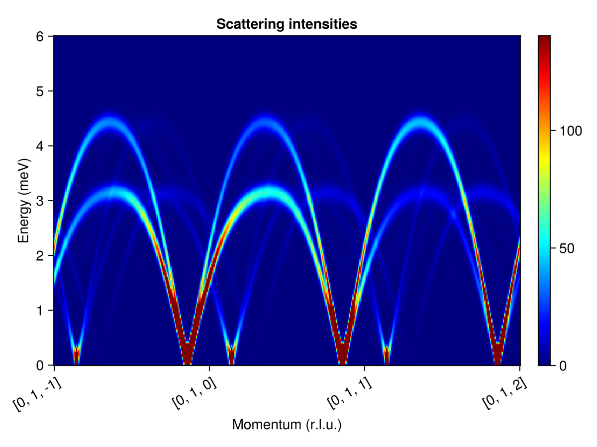
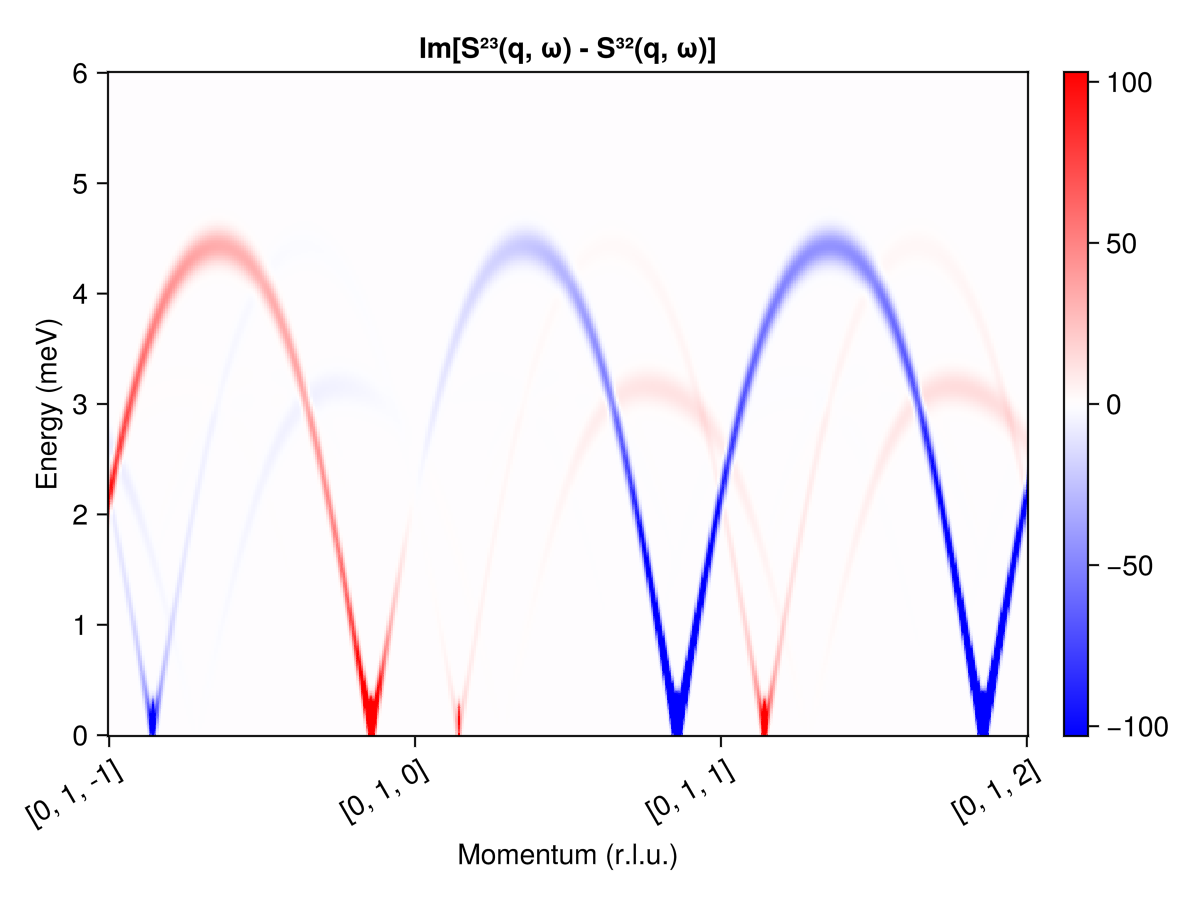
Use ssf_custom_bm to calculate the imaginary part of $\mathcal{S}^{2, 3}(𝐪, ω) - \mathcal{S}^{3, 2}(𝐪, ω)$. In polarized neutron scattering, it is conventional to express the 3×3 structure factor matrix $\mathcal{S}^{α, β}(𝐪, ω)$ in the Blume-Maleev polarization axis system. Specify the scattering plane $[0, K, L]$ via the spanning vectors $𝐮 = [0, 1, 0]$ and $𝐯 = [0, 0, 1]$.
measure = ssf_custom_bm(sys; u=[0, 1, 0], v=[0, 0, 1]) do q, ssf
    imag(ssf[2,3] - ssf[3,2])
end
swt = SpinWaveTheorySpiral(sys; measure, k, axis)
res = intensities(swt, path; energies, kernel=gaussian(fwhm=0.25))
plot_intensities(res; units, saturation=0.8, allpositive=false,
                 title="Im[S²³(q, ω) - S³²(q, ω)]")