Download this example as Julia file or Jupyter notebook.

SW09 - k=0 kagome AFM and DM

This is a Sunny port of SpinW Tutorial 9, originally authored by Bjorn Fak and Sandor Toth. It calculates the spin wave spectrum of the kagome lattice with antiferromagnetic and DM interactions, with ordering wavevector of $𝐤 = 0$, and relative rotation 120° between sublattices

Load Sunny and the GLMakie plotting package

using Sunny, GLMakie, LinearAlgebra

Define the chemical cell of a kagome lattice with spacegroup 147 (P-3).

units = Units(:meV, :angstrom)
latvecs = lattice_vectors(6, 6, 8, 90, 90, 120)
cryst = Crystal(latvecs, [[1/2, 0, 0]], 147)
view_crystal(cryst; ndims=2)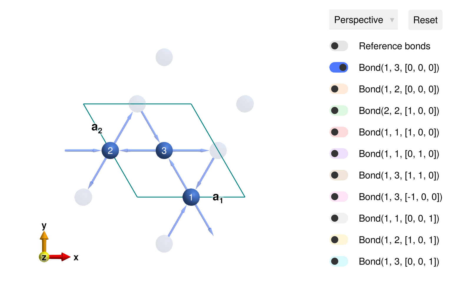

Construct a spin system with antiferromagnetic exchange and a Dzyaloshinskii-Moriya interaction along the first neighbor bond. The symbol I comes from Julia's LinearAlgebra package, and is used to promote the scalar exchange strength 1 meV to a 3×3 exchange matrix. The function dmvec promotes the DM interaction vector $[0, 0, -0.08]$ meV to a 3×3 antisymmetric matrix with nonzero $(x,y)$ components, defined with respect to the global Cartesian coordinate system.

sys = System(cryst, [1 => Moment(s=1, g=2)], :dipole)
J = 1.0*I + dmvec([0, 0, -0.08])

3×3 StaticArraysCore.SMatrix{3, 3, Float64, 9} with indices SOneTo(3)×SOneTo(3):
 1.0   -0.08  -0.0
 0.08   1.0    0.0
 0.0   -0.0    1.0

As in in Tutorial 7, energy minimization determines a $𝐤 = 0$ magnetic order with 120° rotation between the three sublattices.

set_exchange!(sys, J, Bond(2, 3, [0, 0, 0]))
randomize_spins!(sys)
minimize_energy!(sys)
plot_spins(sys; ndims=2)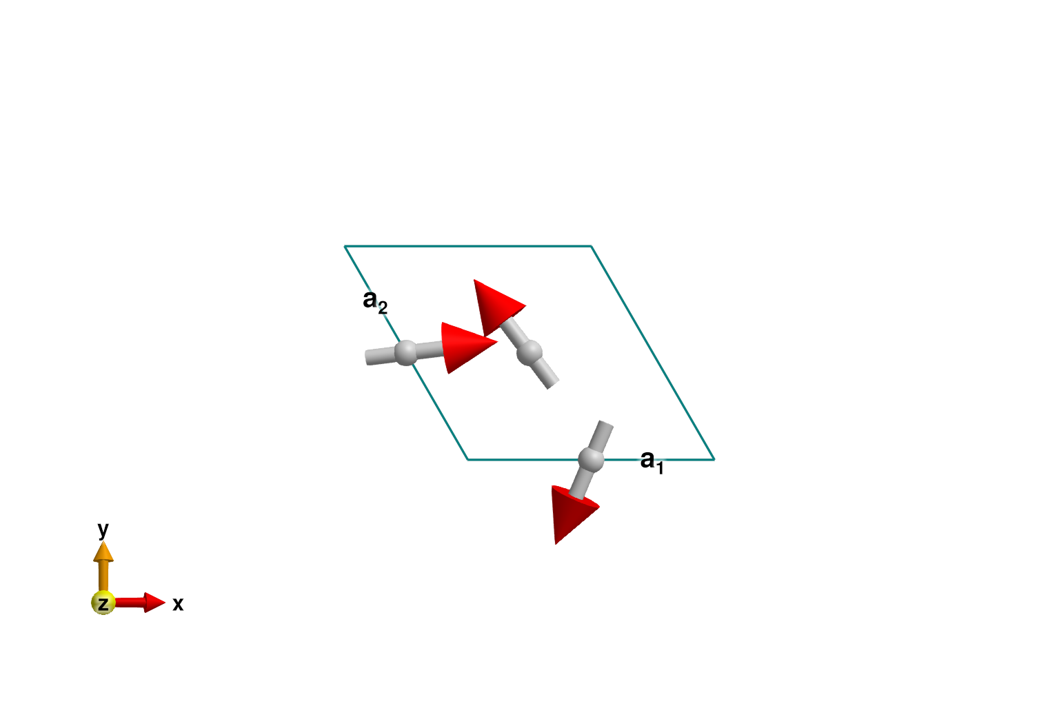

Calculate and plot intensities for a path through $𝐪$-space.

swt = SpinWaveTheory(sys; measure=ssf_perp(sys))
qs = [[-1/2,0,0], [0,0,0], [1/2,1/2,0]]
path = q_space_path(cryst, qs, 400)
res = intensities_bands(swt, path)
plot_intensities(res; units)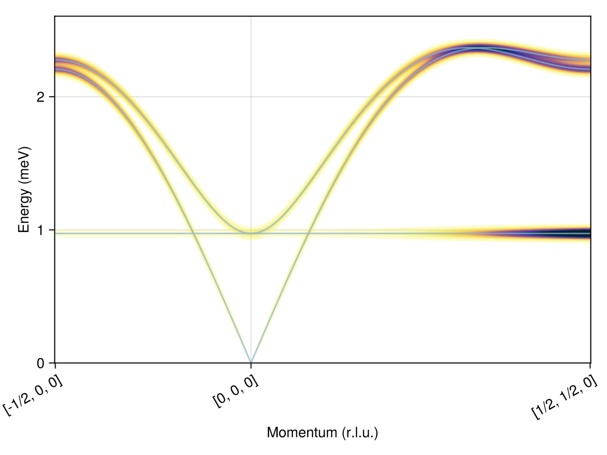

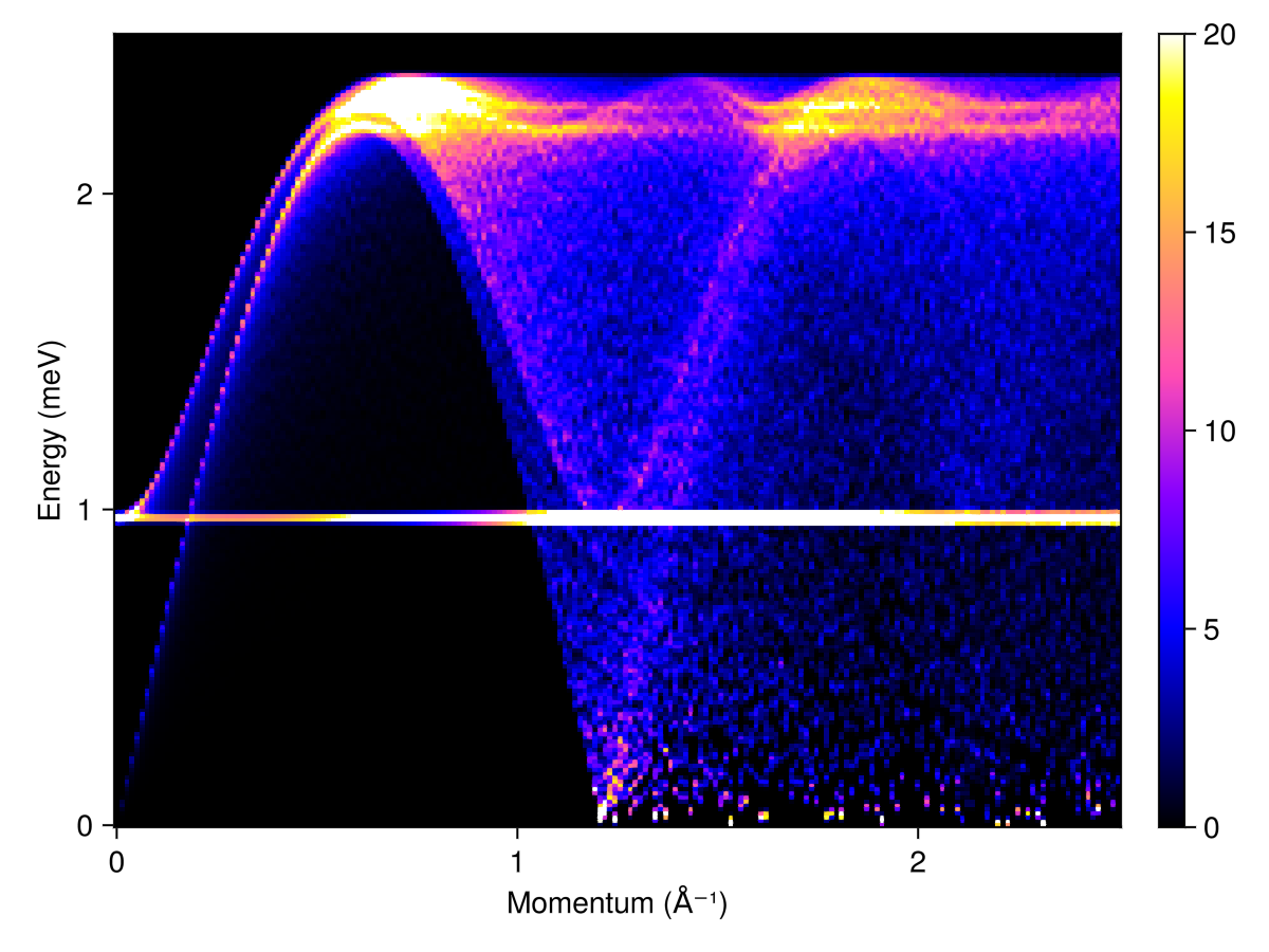
Calculate and plot the powder averaged spectrum. Because the intensities are dominated by a flat band at about 0.97 meV, select an empirical colorrange that brings the lower-intensity features into focus.

radii = range(0, 2.5, 200)
energies = range(0, 2.5, 200)
kernel = gaussian(fwhm=0.02)
res = powder_average(cryst, radii, 1000) do qs
    intensities(swt, qs; energies, kernel)
end
plot_intensities(res; units, colorrange=(0,20))