Download this example as Julia file or Jupyter notebook.
SW13 - LiNiPO₄
This is a Sunny port of SpinW Tutorial 13, originally authored by Sandor Toth. It calculates the spin wave spectrum of LiNiPO₄.
Load packages
using Sunny, GLMakieBuild an orthorhombic lattice and populate the Ni atoms according to Wyckoff 4c of spacegroup 62.
units = Units(:meV, :angstrom)
a = 10.02
b = 5.86
c = 4.68
latvecs = lattice_vectors(a, b, c, 90, 90, 90)
positions = [[1/4, 1/4, 0]]
types = ["Ni"]
cryst = Crystal(latvecs, positions, 62; types)
view_crystal(cryst)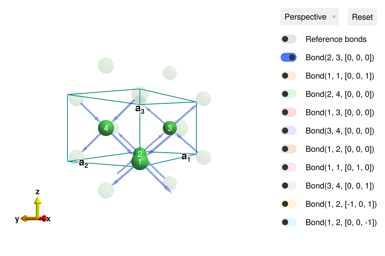
Create a system with exchange parameters taken from T. Jensen, et al., Phys. Rev. B 79, 092413 (2009). The corrected anisotropy values are taken from the thesis of T. Jensen. The mode :dipole_uncorrected avoids a classical-to-quantum rescaling factor of anisotropy strengths, as needed for consistency with the original fits.
sys = System(cryst, [1 => Moment(s=1, g=2)], :dipole_uncorrected)
Jbc =  1.036
Jb  =  0.6701
Jc  = -0.0469
Jac = -0.1121
Jab =  0.2977
Da  =  0.1969
Db  =  0.9097
set_exchange!(sys, Jbc, Bond(2, 3, [0, 0, 0]))
set_exchange!(sys, Jc, Bond(1, 1, [0, 0, -1]))
set_exchange!(sys, Jb, Bond(1, 1, [0, 1, 0]))
set_exchange!(sys, Jab, Bond(1, 2, [0, 0, 0]))
set_exchange!(sys, Jab, Bond(3, 4, [0, 0, 0]))
set_exchange!(sys, Jac, Bond(3, 1, [0, 0, 0]))
set_exchange!(sys, Jac, Bond(4, 2, [0, 0, 0]))
set_onsite_coupling!(sys, S -> Da*S[1]^2 + Db*S[2]^2, 1)
Energy minimization yields a co-linear order along the $c$ axis.
randomize_spins!(sys)
minimize_energy!(sys)
plot_spins(sys; color=[S[3] for S in sys.dipoles])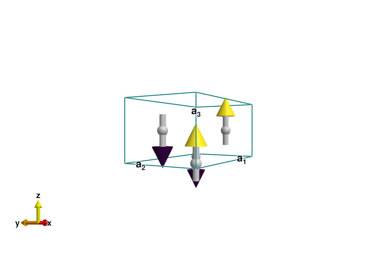
Calculate the spectrum along path [ξ, 1, 0]
swt = SpinWaveTheory(sys; measure=ssf_perp(sys))
qs = [[0, 1, 0], [2, 1, 0]]
path = q_space_path(cryst, qs, 400)
res = intensities_bands(swt, path)
fig = Figure(size=(768, 300))
plot_intensities!(fig[1, 1], res; units)
Makie.Axis with 5 plots:
┣━ Makie.Heatmap{Tuple{Makie.EndPoints{Float64}, Makie.EndPoints{Float64}, Matrix{Float32}}}
┣━ Makie.Lines{Tuple{Vector{GeometryBasics.Point{2, Float64}}}}
┣━ Makie.Lines{Tuple{Vector{GeometryBasics.Point{2, Float64}}}}
┣━ Makie.Lines{Tuple{Vector{GeometryBasics.Point{2, Float64}}}}
┗━ Makie.Lines{Tuple{Vector{GeometryBasics.Point{2, Float64}}}}
There are two physical bands with nonvanishing intensity. To extract these intensity curves, we must filter out the additional bands with zero intensity. One way is to sort the data along dimension 1 (the band index) with the comparison operator "is intensity less than $10^{-12}$". Doing so moves the physical bands to the end of the array axis. Call the Makie lines! function to make a custom plot.
data_sorted = sort(res.data; dims=1, by= >(1e-12))
ax = Axis(fig[1, 2], xlabel="Momentum (r.l.u.)", ylabel="Intensity",
          xticks=res.qpts.xticks, xticklabelrotation=π/6)
lines!(ax, data_sorted[end, :]; label="Lower band")
lines!(ax, data_sorted[end-1, :]; label="Upper band")
axislegend(ax)
fig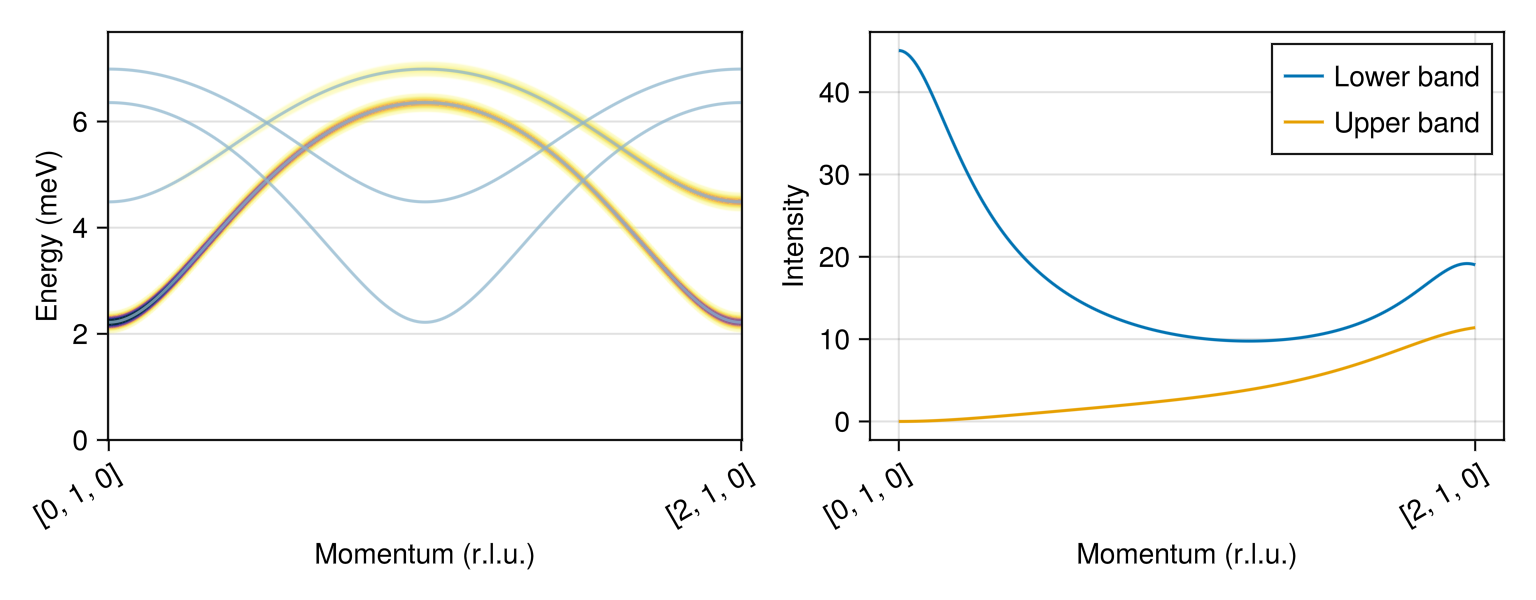
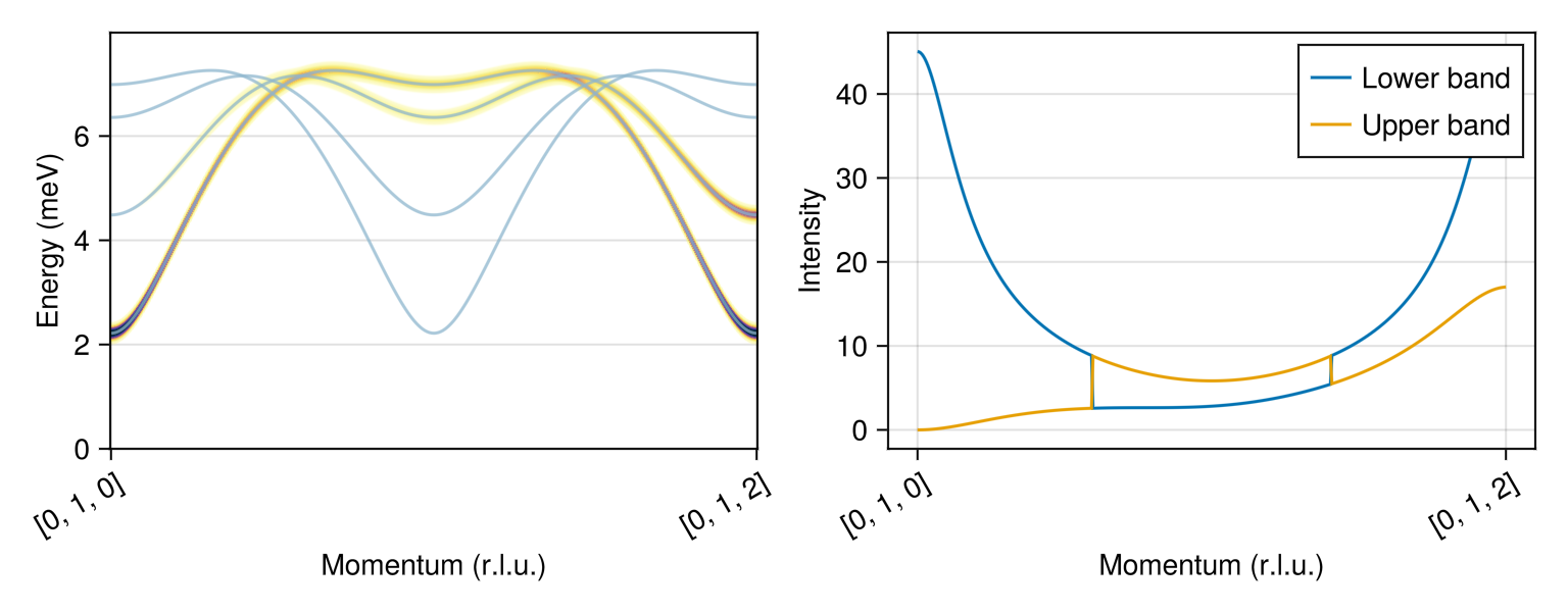
Make the same plots along path [0, 1, ξ]
qs =  [[0, 1, 0], [0, 1, 2]]
path = q_space_path(cryst, qs, 400)
res = intensities_bands(swt, path)
fig = Figure(size=(768, 300))
plot_intensities!(fig[1, 1], res; units)

data_sorted = sort(res.data; dims=1, by=x->abs(x)>1e-12)
ax = Axis(fig[1, 2], xlabel="Momentum (r.l.u.)", ylabel="Intensity",
          xticks=res.qpts.xticks, xticklabelrotation=π/6)
lines!(ax, data_sorted[end, :]; label="Lower band")
lines!(ax, data_sorted[end-1, :]; label="Upper band")
axislegend(ax)
fig