Download this example as Julia file or Jupyter notebook.
SW01 - FM Heisenberg chain
This is a Sunny port of SpinW Tutorial 1, originally authored by Goran Nilsen and Sandor Toth. It calculates the spin wave spectrum of the ferromagnetic Heisenberg nearest-neighbor spin chain.
Load Sunny and the GLMakie plotting package.
using Sunny, GLMakieDefine a chemical cell for the spin chain lattice. It is tetrahedral, with a short dimension of 3 Å and two long dimensions of 8 Å. Observe that Sunny infers the spacegroup 'P 4/m m m' (123).
units = Units(:meV, :angstrom)
a = 3.0
b = 8.0
c = 8.0
latvecs = lattice_vectors(a, b, c, 90, 90, 90)
positions = [[0, 0, 0]]
cryst = Crystal(latvecs, positions)
Crystal
Spacegroup 'P 4/m m m' (123)
Lattice params a=3, b=8, c=8, α=90°, β=90°, γ=90°
Cell volume 192
Wyckoff 1a (site sym. '4/mmm'):
1. [0, 0, 0]
View the crystal in 2D. The nearest neighbor bond along the chain is visible, and labeled Bond(1, 1, [1, 0, 0]). The first two atom indices must be 1, because there is only a single atom in the chemical cell. The vector [1, 0, 0] indicates that the bond includes a displacement of $1 𝐚_1 + 0 𝐚_2 + 0 𝐚_3$ between chemical cells.
view_crystal(cryst; ndims=2, ghost_radius=8)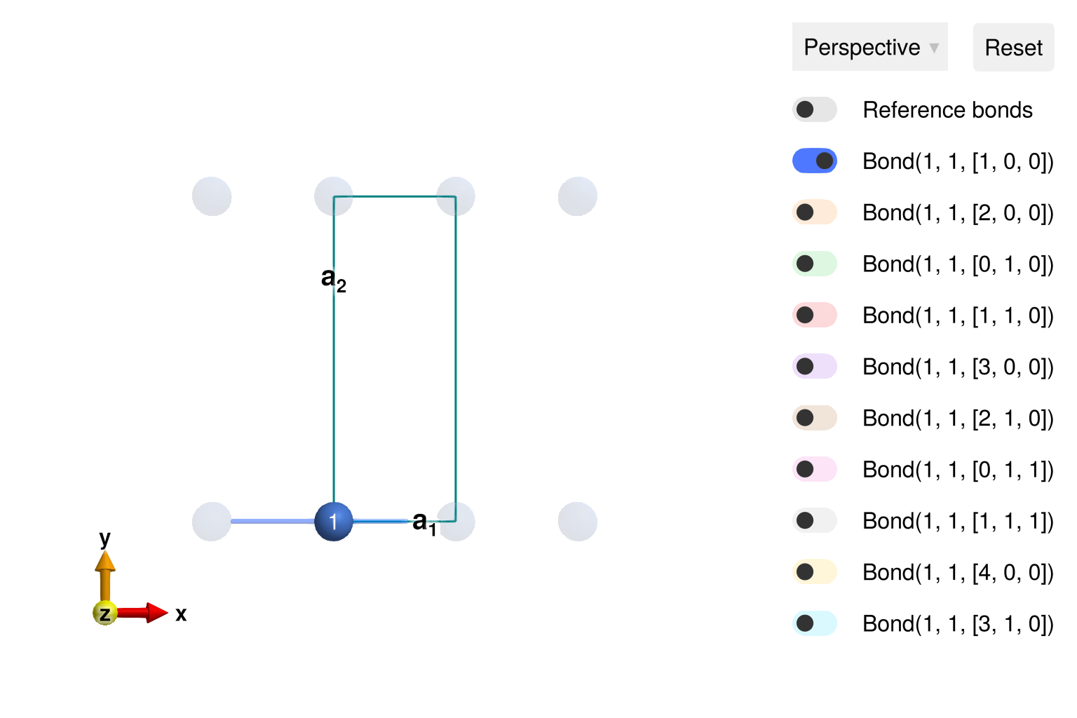
Sunny will always perform symmetry analysis based on the provided crystallographic information. For example, one can see that there are three different symmetry-equivalent classes of bonds up to a distance of 8 Å, and the symmetry-allowed exchange matrices are strongly constrained.
print_symmetry_table(cryst, 8)Atom 1
Position [0, 0, 0], Wyckoff 1a
Allowed g-tensor: [A 0 0
0 B 0
0 0 B]
Allowed anisotropy in Stevens operators:
c₁*(-𝒪[2,0]+3𝒪[2,2]) +
c₂*(𝒪[4,0]+5𝒪[4,2]) + c₃*(𝒪[4,0]+5𝒪[4,4]) +
c₄*(-𝒪[6,0]+21𝒪[6,4]) + c₅*(-(16/231)𝒪[6,0]+(5/11)𝒪[6,2]+𝒪[6,6])
Bond(1, 1, [1, 0, 0])
Distance 3, coordination 2
Connects [0, 0, 0] to [1, 0, 0]
Allowed exchange matrix: [A 0 0
0 B 0
0 0 B]
Bond(1, 1, [2, 0, 0])
Distance 6, coordination 2
Connects [0, 0, 0] to [2, 0, 0]
Allowed exchange matrix: [A 0 0
0 B 0
0 0 B]
Bond(1, 1, [0, 1, 0])
Distance 8, coordination 4
Connects [0, 0, 0] to [0, 1, 0]
Allowed exchange matrix: [A 0 0
0 B 0
0 0 C]Use the chemical cell to create a spin System with spin $s = 1$ and a magnetic form factor for Cu¹⁺. In this case, it is only necessary to simulate a single chemical cell. The option :dipole indicates that, following traditional spin wave theory, we are modeling quantum spins using only their expected dipole moments.
sys = System(cryst, [1 => Moment(s=1, g=2)], :dipole)System [Dipole mode]
Supercell (1×1×1)×1
Energy per site 0
Set a nearest neighbor exchange interaction of $J = -1$ meV between neighboring atoms. That is, the total energy along each bond is $J S_i S_{i+1}$. The exchange interaction will be propagated to all symmetry equivalent bonds in the system.
J = -1
set_exchange!(sys, J, Bond(1, 1, [1, 0, 0]))
Find the energy minimum, which is ferromagnetic. The energy per site is $-J$ for this unfrustrated FM order.
randomize_spins!(sys)
minimize_energy!(sys)
energy_per_site(sys)-1.0Because the interaction is Heisenberg (isotropic), the minimization procedure selects an arbitrary direction in spin-space.
plot_spins(sys; ndims=2, ghost_radius=8)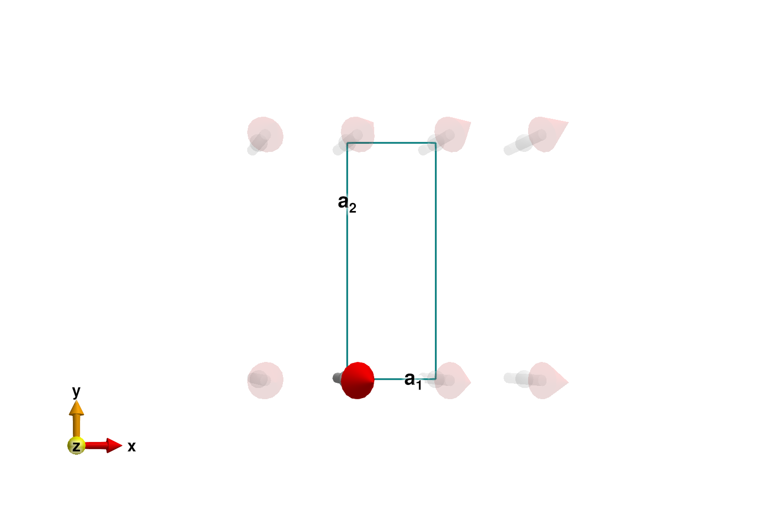
Build a SpinWaveTheory object to measure the dynamical spin-spin structure factor (SSF). Select ssf_perp to project intensities onto the space perpendicular to the momentum transfer $𝐪$, which is appropriate for an unpolarized neutron beam.
swt = SpinWaveTheory(sys; measure=ssf_perp(sys))SpinWaveTheory [Dipole mode]
1 atoms
Define a path from $[0,0,0]$ to $[1,0,0]$ in reciprocal lattice units (RLU) containing 400 sampled $𝐪$-points.
qs = [[0,0,0], [1,0,0]]
path = q_space_path(cryst, qs, 400)
QPath (400 samples)
[0, 0, 0] → [1, 0, 0]
Calculate and plot the intensities along this path.
res = intensities_bands(swt, path)
plot_intensities(res; units)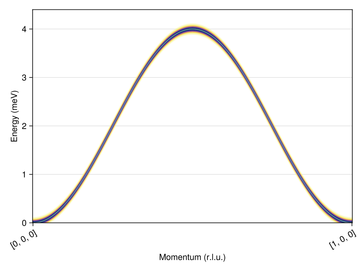
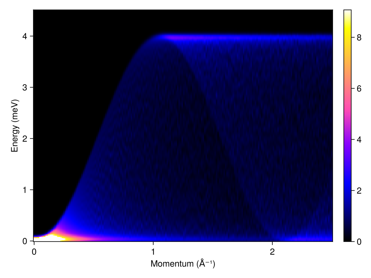
Perform a powder average over the intensities for 200 radii between 0 and 2.5 inverse Å. Each radial distance defines a spherical shell in recripocal space, which will be sampled approximately uniformly, involving 1000 sample points. Measure intensities for 200 energy values between 0 and 5 meV. Gaussian line-broadening is applied with a full-width at half-maximum (FWHM) of 0.1 meV. With the above parameters, this calculation takes about a second on a modern laptop. To decrease stochastic error, one can increase the number of sample points on each spherical shell.
radii = range(0, 2.5, 200) # 1/Å
energies = range(0, 4.5, 200) # meV
kernel = gaussian(fwhm=0.1)
res = powder_average(cryst, radii, 1000) do qs
    intensities(swt, qs; energies, kernel)
end
plot_intensities(res; units)