Download this example as Julia file or Jupyter notebook.

11. Fitting to inelastic powder-averaged data

This tutorial fits an effective spin model for the hyperhoneycomb magnet β-Na₂PrO₃ using inelastic, powder-averaged neutron scattering data. The study follows Okuma et al., Nat. Commun., 15, 10615 (2024).

using Sunny, GLMakie, LinearAlgebra

The Pr ions occupy the single Wyckoff site 16g of spacegroup Fddd. The ions form two families of zigzag chains that run alternatingly along the $a+b$ and $a-b$ diagonals, with inter-chain bonding along $c$.

units = Units(:meV, :angstrom)
latvecs = lattice_vectors(6.74560, 9.74653, 20.4972, 90, 90, 90)
positions = [[1/8, 1/8, 0.7087]]
cryst = Crystal(latvecs, positions, 70)

Crystal
Spacegroup 'F d d d' (70)
Lattice params a=6.746, b=9.747, c=20.5, α=90°, β=90°, γ=90°
Cell volume 1348
Wyckoff 16g (site sym. '..2'):
   1. [5/8, 1/8, 0.04130]
   2. [1/8, 5/8, 0.04130]
   3. [5/8, 1/8, 0.2087]
   4. [1/8, 5/8, 0.2087]
   5. [3/8, 3/8, 0.2913]
   6. [7/8, 7/8, 0.2913]
   7. [3/8, 3/8, 0.4587]
   8. [7/8, 7/8, 0.4587]
   9. [1/8, 1/8, 0.5413]
   10. [5/8, 5/8, 0.5413]
   11. [1/8, 1/8, 0.7087]
   12. [5/8, 5/8, 0.7087]
   13. [7/8, 3/8, 0.7913]
   14. [3/8, 7/8, 0.7913]
   15. [7/8, 3/8, 0.9587]
   16. [3/8, 7/8, 0.9587]

The magnetic unit cell coincides with the crystallographic primitive cell. Reducing the system to just four Pr ions will accelerate the calculations.

sys = System(cryst, [1 => Moment(s=1/2, g=0.94)], :dipole)
sys = reshape_supercell(sys, primitive_cell(cryst))

System [Dipole mode]
Supercell (1×1×1)×4
Reshaped cell [  0 1/2 1/2
               1/2   0 1/2
               1/2 1/2   0]
Energy per site 0

Label the effective spin interactions in the language of the compass model. The expressions come from "Supplementary Note 4" of the Okuma et al. paper.

Each Pr ion is surrounded by an O₆ octahedron, which defines a natural local frame. The rotation matrix $R$ maps from the global Cartesian frame to this local frame.

R = [-1/√2 0 -1/√2; 1/√2 0 -1/√2; 0 -1 0]

Nearest-neighbor bonds connecting different zigzag chains are the "z-bonds" of the compass-model. Label coupling strengths $(J, Γ, K)$. For example, the notation :J => 0.0 assigns the symbol :J to the Heisenberg coupling and initializes its strength to zero. Labeled parameters can be modified using, e.g., set_params!.

zbond = Bond(1, 3, [0, 0, 0])
set_exchange!(sys, 1.0, zbond, :J => 0.0)
set_exchange!(sys, R' * [0 1 0; 1 0 0; 0 0 0] * R, zbond, :Γ => 0.0)
set_exchange!(sys, R' * [0 0 0; 0 0 0; 0 0 1] * R, zbond, :K => 0.0)

Nearest-neighbor bonds within each zigzag chain are the "x-bonds" and "y-bonds" of the compass-model. Their equivalence is fixed by Fddd spacegroup symmetries. Label coupling strengths $(J', Γ', K')$.

xbond = Bond(3, 5, [0, 0, 0])
set_exchange!(sys, 1.0, xbond, :J′ => 0.0)
set_exchange!(sys, R' * [0 0 0; 0 0 1; 0 1 0] * R, xbond, :Γ′ => 0.0)
set_exchange!(sys, R' * [1 0 0; 0 0 0; 0 0 0] * R, xbond, :K′ => 0.0)

The model ansatz sets $K = K' = 0$. Four parameters are left for fitting.

labels = [:J, :Γ, :J′, :Γ′]

Okuma et al. deduced that the constraints $J = J' > 0$ and $Γ = -Γ' < 0$ produce a magnetic order consistent with diffraction data. Guess some parameters of this form. Energy minimization yields antiferromagnetic (AFM) order along each zigzag chain, with some relative canting between chains. The primitive cell is shown as a gray parallelpiped within the larger orthorhombic cell.

set_params!(sys, labels, [0.9, -0.5, 0.9, +0.5])
randomize_spins!(sys)
minimize_energy!(sys)
plot_spins(sys; ghost_radius=6)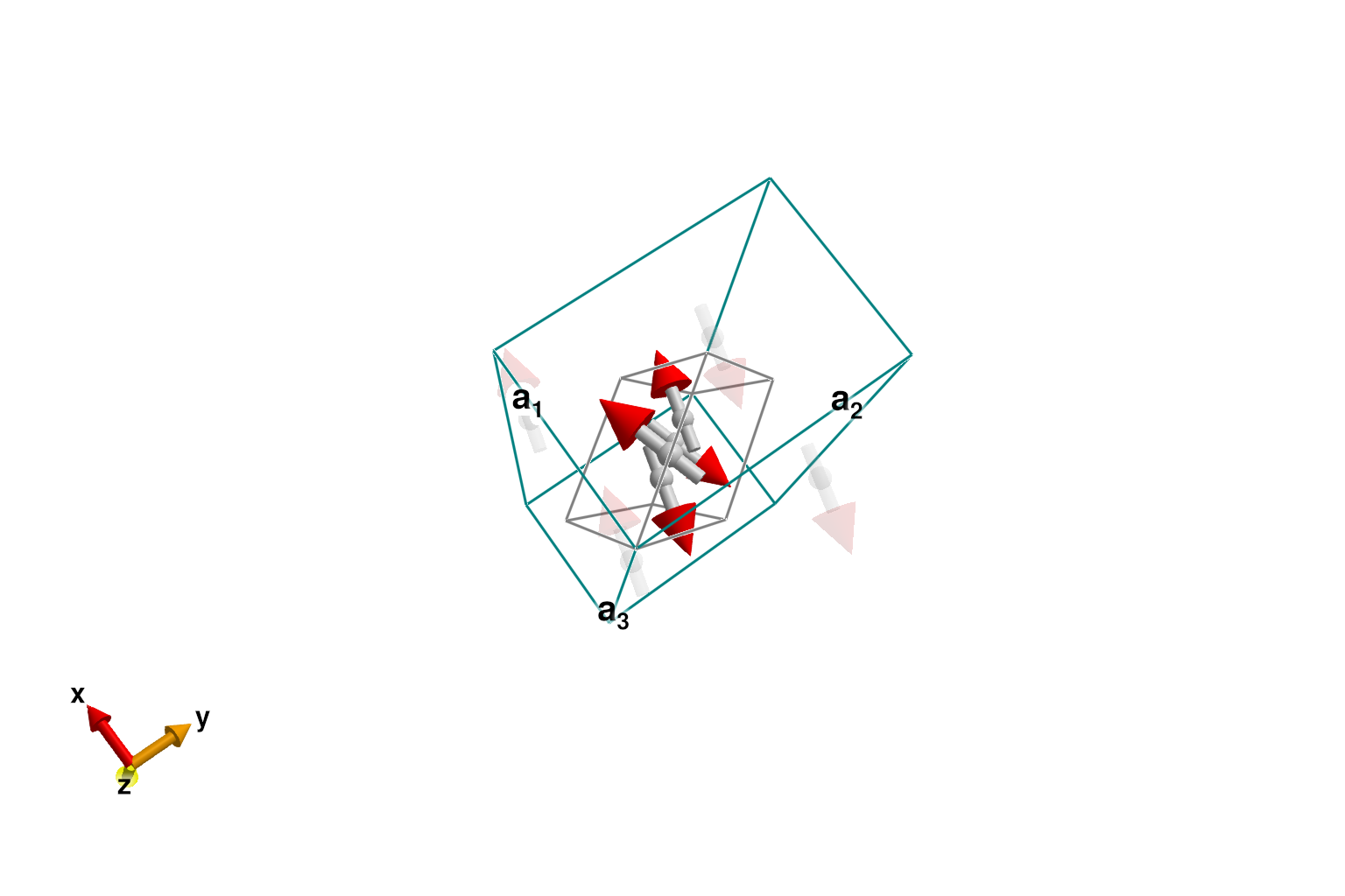

The energy-minimized dipoles of the primitive cell can be directly inspected. Their Cartesian coordinates are also available with global_positions. Sites 1 and 4 belong to one zigzag chain, while sites 2 and 3 belong to the other.

vec(sys.dipoles)

4-element Vector{StaticArraysCore.SVector{3, Float64}}:
 [-0.4811252243246277, -0.13608276348816822, -5.45199628737701e-13]
 [0.4811252243247104, -0.1360827634878757, 2.4151924664993077e-13]
 [-0.4811252243245497, 0.13608276348844398, -8.211597156268711e-13]
 [0.48112522432479016, 0.1360827634875936, 1.5182146474162355e-13]

It is easiest to visualize the magnetic structure in the context of a chemical unit cell. Do so by passing sys to view_crystal. To see the spins, toggle from "No dipoles" to "Spin dipoles". To see all edges of the hyperhoneycomb lattice, toggle on bonds (3, 5) and (1, 3). The symmetric exchange tensor along each bond is depicted as an ellipsoid; its elongations are a visual representation of the anisotropic coupling strengths.

view_crystal(sys)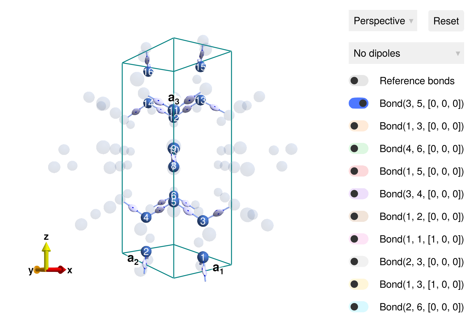

To simplify the tutorial, we will fit to powder data on a coarse grid of just 30 momenta and 100 energies. The original data is available online and has far higher resolution.

ref_data = [NaN NaN NaN NaN NaN NaN NaN NaN NaN NaN NaN NaN NaN NaN NaN NaN NaN NaN NaN NaN NaN NaN NaN NaN NaN NaN NaN NaN NaN NaN; NaN NaN NaN NaN NaN NaN NaN NaN NaN NaN NaN NaN NaN NaN NaN NaN NaN NaN NaN NaN NaN NaN NaN NaN NaN NaN NaN NaN NaN NaN; NaN NaN NaN NaN NaN NaN NaN NaN NaN NaN NaN NaN NaN NaN NaN NaN NaN NaN NaN NaN NaN NaN NaN NaN NaN NaN NaN NaN NaN NaN; NaN NaN NaN NaN NaN NaN NaN NaN NaN NaN NaN NaN NaN NaN NaN NaN NaN NaN NaN NaN NaN NaN NaN NaN NaN NaN NaN NaN NaN NaN; NaN NaN NaN NaN NaN NaN NaN NaN NaN NaN NaN NaN NaN NaN NaN NaN NaN NaN NaN NaN NaN NaN NaN NaN NaN NaN NaN NaN NaN NaN; -204.56 -90.67 -5.11 -12.45 -9.22 -30.89 3.31 -3.46 -13.85 84.12 -16.41 11.02 16.19 -37.38 42.03 6.27 -15.1 49.02 42.69 9.4 -45.59 7.69 29.71 47.83 44.31 2.09 29.61 -2.58 12.24 9.34; 32.29 -10.59 8.68 3.79 -19.86 11.91 -0.6 11.5 8.22 15.71 8.24 -8.84 7.01 27.85 6.73 22.49 -10.55 23.04 6.86 0.08 11.72 10.96 0.29 13.36 1.62 22.77 10.19 21.25 0.24 0.55; 43.76 38.36 33.94 2.38 -7.6 1.39 -5.87 -6.54 -4.86 22.79 4.28 -7.4 6.69 0.15 0.22 12.96 7.48 15.96 0.29 16.99 8.24 10.59 -1.75 -0.01 13.33 0.11 0.23 0.07 -0.05 14.3; 60.42 -1.59 8.72 -0.65 2.5 19.1 0.67 15.14 -2.34 7.27 27.43 9.68 0.01 0.09 0.87 12.07 0.18 0.74 -0.04 0.03 0.15 0.15 0.44 0.03 0.1 0.06 0.18 0.32 0.11 0.31; -9.54 16.78 17.69 4.91 21.08 -1.07 8.88 -4.66 -3.12 4.57 0.73 6.63 0.39 0.09 0.13 0.02 0.06 0.21 0.26 0.19 0.02 0.01 0.47 0.2 0.13 0.1 0.16 0.08 0.08 0.25; 17.64 27.41 9.98 -2.43 14.34 16.62 -0.63 11.96 -3.95 4.45 14.77 0.24 0.09 0.08 -0.08 0.12 0.01 0.02 0.03 0.08 0.05 0.05 0.06 0.04 0.11 0.04 0.18 0.03 0.04 -0.3; 14.22 12.29 -1.43 -6.0 7.39 -7.13 -11.5 -12.2 -0.36 0.85 3.74 0.49 0.24 0.07 0.05 0.15 0.38 0.06 0.07 0.05 0.03 0.15 0.04 0.03 0.03 -0.0 0.03 0.07 0.14 0.15; 1.8 2.56 5.2 6.88 11.24 2.17 -1.92 5.62 6.07 9.3 1.37 0.05 0.29 0.08 0.04 0.05 0.03 0.17 0.03 0.06 0.05 0.0 0.03 0.03 0.04 0.07 0.04 0.03 0.05 0.03; 34.56 -3.57 -6.25 8.8 7.26 6.52 1.16 0.35 2.52 0.77 4.99 0.1 0.15 0.05 0.06 0.15 0.12 0.05 0.01 0.03 0.15 0.03 -0.01 -0.0 0.04 0.06 0.13 0.04 0.0 0.1; 0.11 18.57 10.8 8.63 9.79 -3.78 6.0 6.52 0.51 1.01 0.15 0.25 0.15 -0.02 0.03 0.1 0.04 0.04 0.05 0.01 0.06 0.01 0.03 0.04 0.0 0.03 0.04 0.01 0.02 0.04; 20.59 7.72 5.53 7.25 4.55 -1.04 -1.16 -1.21 0.07 1.23 -0.43 0.15 0.1 0.03 0.03 0.04 0.01 0.04 0.06 0.02 0.08 0.01 0.0 0.03 0.01 -0.01 0.02 0.01 0.06 0.07; 23.11 2.88 14.73 4.6 2.47 0.62 0.38 4.49 0.91 5.07 0.16 0.0 0.15 0.06 -0.01 0.04 0.07 0.02 0.05 0.02 0.03 0.01 0.16 0.01 0.02 0.03 0.04 0.02 -0.01 0.13; 0.16 0.13 0.18 7.41 8.63 0.99 3.88 8.77 3.56 6.27 0.71 0.1 0.08 -0.0 0.01 0.06 0.13 0.02 0.03 0.03 0.01 0.03 0.04 0.07 0.02 0.06 0.1 0.03 -0.0 0.03; -0.01 14.14 9.06 8.63 7.31 2.28 -0.01 0.33 1.0 0.24 0.77 0.06 0.18 -0.0 0.02 0.06 0.07 0.04 0.01 0.04 0.05 0.05 0.03 0.01 0.01 0.04 0.04 0.02 0.05 0.05; 0.08 10.63 1.96 0.39 4.0 -0.17 4.82 -3.67 1.31 6.84 0.21 0.06 0.14 0.01 0.04 0.04 0.01 0.03 0.05 0.09 0.0 0.03 0.03 0.04 0.01 -0.0 0.02 0.07 0.01 0.11; -0.05 11.91 4.86 12.63 9.68 6.26 -4.81 6.51 9.31 0.63 0.24 0.16 -0.02 0.01 0.02 0.11 0.05 0.06 0.02 0.01 -0.01 0.01 0.05 0.07 0.02 0.02 0.08 0.03 0.06 0.08; -13.95 -10.0 3.1 2.31 7.55 9.38 7.28 8.87 3.99 3.61 -1.29 -5.53 -5.11 -2.0 0.3 -6.07 4.5 -2.88 -0.59 0.05 1.69 -1.2 0.99 -1.78 0.14 1.22 -0.82 -3.35 -6.63 1.08; -34.2 0.61 -6.3 -9.21 -0.68 3.84 5.69 3.53 5.76 4.42 -0.39 -2.03 1.46 -10.74 -4.25 -0.59 -1.9 -3.27 0.1 -0.12 -4.5 -2.22 -6.26 6.0 -3.76 -6.0 -2.02 4.0 0.73 -3.06; -37.93 6.94 -3.89 -1.97 -3.0 -2.59 -1.59 -6.12 -3.54 1.74 -6.39 -5.87 -6.54 -9.86 -8.66 -7.01 -10.47 -9.81 -1.05 0.19 -5.33 1.41 -8.17 -6.81 1.38 -2.37 -7.85 -7.02 -6.62 -1.79; -36.19 -9.66 -9.4 -4.68 -1.41 -0.66 -7.47 -4.96 -3.31 -3.49 -5.29 -3.06 -2.61 -1.13 -0.0 -1.91 -3.67 2.26 -2.45 -7.29 -6.18 -6.3 -6.41 -2.35 -7.29 -11.51 -4.13 -6.66 -4.57 -10.65; -22.16 -8.1 -1.75 1.54 -6.66 -10.16 -7.11 5.77 -3.43 1.52 -8.27 -6.96 -1.82 -7.21 -8.85 -7.45 3.64 -5.25 -0.78 -2.79 -9.89 -8.77 -3.67 -12.61 -6.53 -10.15 -12.71 -3.45 3.05 -3.15; -5.95 -14.74 -7.74 -3.36 -3.65 -4.13 -6.71 -10.53 -4.81 -4.85 -2.8 4.76 -2.72 -3.89 2.31 -8.25 -10.41 -11.3 -11.51 -5.2 3.98 -12.95 -13.39 -3.34 -13.12 -11.89 -13.76 -3.7 -5.74 -7.86; -18.16 0.81 -5.75 -2.28 -12.74 -9.95 -1.16 -4.6 -11.18 -9.79 0.63 -9.06 -9.6 -5.52 -9.27 -3.32 -9.68 -5.95 -9.54 -10.71 -6.82 -1.13 -3.86 -7.89 -9.16 -0.4 -2.21 -8.68 -7.41 -10.68; -65.45 -29.31 -19.77 -16.11 -6.9 -6.61 -10.75 -14.29 -12.7 -12.4 -6.64 -10.47 -6.7 -11.88 -16.74 -17.29 -9.76 -6.36 -4.23 -6.32 -17.27 -7.43 -12.11 -7.59 2.22 -7.34 -9.87 -5.95 -10.12 -18.18; -85.68 -22.63 -16.77 -17.9 -6.62 -8.05 -9.55 -16.74 -12.19 -11.78 -14.85 -2.36 -9.68 -13.45 -5.16 -10.37 -7.17 -2.04 -6.2 -8.61 -13.15 -9.2 -16.15 -13.27 -6.95 -9.4 -15.18 -9.47 -7.48 -17.79; -45.18 -31.49 -12.56 -11.01 -15.53 -11.67 -6.11 -10.53 -21.07 -13.9 -10.58 -6.97 -7.57 -8.48 0.22 3.06 -9.71 -8.34 -9.51 -4.99 -15.72 -5.74 -6.58 -10.01 -5.19 -4.88 -11.74 -9.07 -3.25 -7.0; -84.13 -30.58 -1.86 -17.18 -3.89 -9.84 -6.57 -5.66 -13.6 -13.04 -8.32 -18.88 -8.4 -18.15 0.26 -8.66 -5.36 -3.08 7.02 -0.12 -15.43 -10.33 -11.51 -10.2 3.74 0.32 -8.1 -12.4 -2.73 -7.36; -84.41 -30.35 -1.24 -13.31 -5.66 -5.07 -1.1 -17.34 -17.01 -18.89 -13.86 -4.42 -16.97 -16.04 11.11 -5.21 4.89 9.68 18.34 -4.41 -13.88 -15.28 -5.71 -8.47 7.45 6.97 -11.57 -9.35 -8.74 -15.48; -52.56 -22.22 -14.24 -0.05 -10.35 -13.15 -9.07 -4.56 -6.53 -11.08 -10.69 -8.74 2.46 -2.01 17.2 9.81 18.47 32.39 34.73 20.34 -11.43 -19.43 -10.35 -0.09 11.54 11.41 -0.42 -13.27 -3.85 -6.7; NaN -27.85 -6.82 -9.91 -10.88 -14.72 -7.59 -2.73 -3.49 -4.67 -18.12 -14.23 -4.32 -5.75 33.64 18.19 8.56 43.57 57.34 23.64 -12.83 -3.26 -5.28 -4.29 17.32 7.61 12.26 5.28 8.67 1.75; NaN -26.43 -1.75 -6.98 -1.38 5.08 3.16 -5.54 -18.05 -10.97 -3.13 -15.48 2.06 0.77 36.6 35.84 40.41 63.08 44.96 35.0 -0.01 -3.79 -0.21 9.7 15.3 18.72 14.99 2.89 6.61 9.08; NaN -26.01 -8.86 -13.49 -3.68 5.7 1.87 -1.66 -10.46 -14.02 -15.64 -5.48 10.42 31.68 41.19 44.41 35.66 78.13 52.66 52.03 -5.27 -7.11 -6.01 8.81 27.24 22.29 13.93 5.72 -0.8 9.95; NaN -29.86 -18.64 -7.16 -0.95 -2.21 -3.53 -6.39 -2.29 -18.52 -0.36 -3.48 3.68 41.81 39.67 39.12 78.36 81.7 83.29 49.35 5.62 -10.63 2.45 27.21 23.36 22.98 16.86 21.37 11.5 17.09; NaN 4.51 -9.83 -2.09 5.34 15.81 -2.64 3.45 -11.48 -9.05 -13.48 -9.77 7.01 30.51 60.62 37.96 73.91 98.36 61.56 62.7 17.74 -3.39 7.26 31.07 38.5 21.88 27.75 32.71 18.27 29.2; NaN 11.23 -6.46 -8.4 4.65 13.4 9.74 -2.55 -6.47 -0.45 -4.65 3.29 30.54 45.61 63.26 85.96 91.99 117.3 78.92 57.74 19.98 -3.75 0.39 34.17 24.71 37.57 34.07 42.78 12.31 6.35; NaN 4.12 -22.88 0.71 6.74 18.24 7.36 14.26 -17.62 -14.94 -11.78 19.33 38.68 47.82 46.64 103.14 129.83 142.67 79.58 60.19 34.6 7.24 26.2 40.44 50.01 47.65 33.9 36.6 28.61 13.89; NaN 19.9 -0.6 6.22 8.42 14.58 12.08 3.7 -7.06 -9.35 -19.71 23.67 32.89 46.94 64.1 68.99 94.89 110.72 82.54 76.52 24.71 10.61 32.14 45.82 31.29 46.72 37.99 13.66 5.67 38.43; NaN 39.57 -0.92 -2.53 12.91 13.23 1.31 12.19 -5.11 -4.38 -10.0 20.73 28.98 51.61 44.15 92.65 162.59 88.03 86.78 89.72 34.02 28.8 34.52 28.75 42.28 51.38 44.97 40.61 45.71 40.45; NaN 68.6 10.91 11.98 27.05 4.82 18.65 -0.96 -8.92 -7.87 -5.39 4.95 33.66 57.97 71.8 128.05 180.39 147.05 101.74 69.99 31.97 42.11 40.46 12.26 42.95 56.04 60.25 41.03 8.92 28.12; NaN 119.35 4.39 -1.85 10.27 8.43 11.45 -1.7 -1.67 -2.94 16.17 17.0 47.15 58.47 86.98 140.36 164.17 122.71 121.16 83.06 36.4 37.61 47.91 57.55 38.52 36.77 50.08 54.48 54.25 47.07; NaN 168.68 49.71 8.73 11.89 18.9 6.26 8.85 -1.26 -4.5 -5.28 9.6 38.36 53.05 89.01 145.37 181.79 142.02 99.58 84.02 53.75 70.26 53.47 48.58 42.64 44.57 60.9 64.1 60.56 37.61; NaN 322.47 64.31 14.66 36.94 11.89 12.93 16.54 -4.46 -14.46 32.61 40.94 36.9 81.31 127.27 210.74 209.43 137.56 104.04 106.12 65.17 68.7 49.57 37.88 50.11 52.33 53.9 57.67 56.95 66.31; NaN 252.5 151.21 34.17 27.82 9.21 6.01 4.42 1.77 -12.88 27.16 49.1 70.5 88.59 123.13 213.28 169.04 119.81 118.74 100.16 84.59 95.29 79.63 44.56 59.75 42.44 66.87 59.83 73.78 59.25; NaN 348.36 195.67 56.48 24.86 9.89 19.38 21.18 3.07 3.29 27.64 49.43 67.9 105.83 149.75 243.94 179.06 156.44 126.12 107.43 147.21 111.14 76.46 69.01 46.97 71.72 70.62 97.61 70.47 89.53; NaN 391.96 293.27 93.94 38.0 13.62 31.99 19.36 13.67 19.56 39.25 47.93 109.55 130.67 177.23 229.54 226.8 167.65 145.47 121.86 150.21 163.81 121.78 61.06 66.05 87.8 81.34 113.35 71.4 106.81; NaN 429.05 357.26 148.56 50.9 28.73 34.71 26.45 20.23 40.08 43.72 56.65 98.16 104.94 224.09 270.53 230.15 180.14 132.06 149.06 182.68 169.72 118.46 87.82 89.63 82.84 75.19 96.37 76.44 109.53; NaN 424.36 383.94 243.56 75.18 26.31 45.25 38.49 51.07 44.13 56.52 73.69 129.03 194.55 225.39 264.6 264.82 206.8 193.63 149.99 210.09 216.39 116.64 82.84 79.1 90.72 94.43 111.67 108.61 134.49; NaN 416.13 463.8 314.56 95.47 49.12 49.73 54.63 73.84 71.35 86.84 94.34 134.89 227.92 269.55 292.14 238.78 231.81 196.68 159.63 216.27 223.18 161.26 141.29 126.73 116.81 114.85 149.93 163.3 168.33; NaN NaN 418.27 362.22 179.17 83.97 56.85 82.45 89.33 72.66 96.64 144.13 206.95 272.45 349.65 339.59 298.52 246.56 242.46 216.86 283.6 278.47 207.44 184.0 146.04 149.11 131.97 143.49 158.19 213.08; NaN NaN 460.54 396.22 275.88 125.94 95.55 103.89 134.52 124.88 135.93 160.91 198.18 366.65 372.78 340.45 354.41 304.2 260.23 287.58 307.35 317.54 257.39 201.47 195.57 158.19 176.03 181.17 188.83 220.39; NaN NaN 520.35 423.4 361.31 200.79 141.12 154.6 176.31 162.13 134.78 212.7 291.83 421.08 532.31 437.21 359.04 352.93 371.91 347.45 397.66 315.22 278.42 307.8 223.74 230.19 226.9 226.52 193.81 265.42; NaN NaN 499.7 455.6 449.82 313.42 209.97 223.29 201.59 181.63 213.75 251.39 345.0 492.37 534.78 470.1 373.13 378.45 432.26 447.94 397.12 376.29 394.2 284.77 251.12 249.28 237.72 260.5 249.13 198.96; NaN NaN 509.02 471.9 432.76 416.62 294.92 224.68 210.31 211.93 227.2 306.59 407.24 461.16 554.51 449.92 388.96 392.83 468.21 429.9 386.53 377.08 382.99 292.86 286.28 255.53 231.72 244.45 295.99 281.44; NaN NaN 414.69 440.78 437.86 421.19 323.02 244.7 194.5 223.41 254.35 334.25 340.16 441.47 469.92 474.73 435.02 404.95 446.13 437.54 386.73 391.32 298.1 313.22 307.17 221.98 263.67 267.4 307.77 149.78; NaN NaN 416.79 530.35 429.01 437.75 358.07 234.67 200.25 229.02 307.18 364.83 415.39 407.81 441.13 497.9 426.04 436.32 481.9 430.93 412.84 362.11 314.05 284.16 254.25 236.54 265.33 253.77 305.14 163.57; NaN NaN 288.18 532.63 424.05 407.47 325.89 240.04 231.99 238.53 352.58 338.4 389.37 362.34 374.77 495.36 417.24 437.13 436.48 366.18 336.41 321.83 301.71 310.35 319.2 287.04 272.33 267.6 278.27 213.18; NaN NaN 198.68 488.65 411.06 365.62 303.69 232.6 217.19 234.06 291.76 338.81 338.02 341.19 351.49 355.73 391.59 394.63 400.91 328.74 268.96 308.71 239.44 279.93 205.05 261.02 252.36 237.24 264.32 280.32; NaN NaN 115.91 378.17 405.26 288.79 280.75 210.85 213.56 215.55 257.96 302.86 354.91 335.04 273.96 311.48 355.99 302.5 276.0 251.75 241.21 275.24 165.71 234.44 241.58 265.03 227.19 195.85 219.06 207.48; NaN NaN 94.45 287.03 377.45 298.1 268.78 205.33 184.04 243.42 273.77 258.75 297.41 321.65 240.56 281.02 367.19 281.03 268.0 222.7 205.03 216.72 182.93 210.68 199.84 222.37 208.23 186.2 212.86 -4.91; NaN NaN 50.26 184.99 384.74 258.81 245.65 239.81 207.13 223.3 281.68 236.0 297.32 268.94 225.43 285.59 333.59 252.65 295.67 196.88 156.8 208.39 204.04 202.64 218.42 176.59 215.89 209.16 204.12 NaN; NaN NaN 75.73 167.97 359.3 274.95 262.67 238.59 227.69 228.21 243.57 297.63 288.41 235.45 208.73 230.96 358.15 256.67 268.02 150.3 222.9 190.73 178.39 207.39 172.0 208.9 191.29 160.32 173.14 NaN; NaN NaN 10.34 90.27 386.39 289.96 254.33 249.63 209.75 262.2 274.07 295.33 248.48 246.74 246.51 242.8 288.29 255.82 270.18 190.59 149.2 165.01 162.91 188.22 172.75 242.43 200.7 205.38 188.63 NaN; NaN NaN NaN 90.24 302.36 341.15 255.07 297.03 276.25 297.36 312.92 308.78 296.74 311.97 289.69 310.0 284.05 255.61 273.91 185.32 172.13 158.18 163.91 209.6 177.95 209.54 206.39 193.0 190.5 NaN; NaN NaN NaN 78.83 263.83 389.46 308.12 295.87 315.06 315.03 276.57 273.29 254.61 249.11 278.34 298.3 294.57 295.27 188.98 168.55 156.24 178.67 183.55 189.26 182.2 210.97 195.08 191.13 208.72 NaN; NaN NaN NaN 73.4 156.29 374.9 335.99 294.46 322.12 326.61 340.88 323.2 213.53 297.86 272.14 236.63 238.31 287.35 231.15 236.92 159.25 176.47 169.0 200.4 176.54 197.19 222.58 227.07 181.75 NaN; NaN NaN NaN 66.52 107.76 355.79 358.6 304.55 347.92 328.22 397.49 340.07 237.83 246.46 251.71 219.86 194.83 261.67 231.51 227.17 190.26 186.15 180.17 190.57 162.7 222.46 219.75 209.56 200.69 NaN; NaN NaN NaN 51.11 119.96 249.56 384.76 355.91 349.6 413.58 391.91 319.98 264.87 210.26 275.11 184.13 191.79 203.28 229.14 198.51 187.18 162.18 161.18 143.83 193.05 217.26 213.05 195.0 94.08 NaN; NaN NaN NaN 67.59 91.96 207.12 373.64 367.62 402.54 480.11 416.52 315.79 283.04 261.14 201.43 151.62 202.59 225.01 201.64 189.96 211.75 202.74 155.81 161.17 193.22 220.0 208.75 209.63 176.73 NaN; NaN NaN NaN 52.95 107.13 192.7 360.65 377.01 428.19 502.02 387.57 298.23 281.03 255.04 222.73 224.78 193.9 181.44 205.08 242.51 207.21 162.82 182.76 168.17 184.67 214.11 260.01 201.34 96.81 NaN; NaN NaN NaN 74.47 94.74 145.41 297.49 437.94 485.81 491.69 358.29 307.15 293.02 244.98 184.77 163.16 147.98 159.9 249.07 211.86 245.36 184.34 163.46 227.71 192.03 231.25 191.49 191.4 53.82 NaN; NaN NaN NaN 102.62 105.37 135.24 262.55 433.68 484.56 420.89 349.14 327.71 267.65 204.28 151.82 172.48 152.72 137.38 188.0 185.22 181.56 155.59 167.32 173.1 185.26 203.85 155.29 207.94 37.43 NaN; NaN NaN NaN 123.97 114.47 103.53 184.06 372.33 375.15 314.98 296.84 246.42 165.12 190.54 174.33 174.63 196.1 144.38 106.72 165.69 216.16 137.5 176.99 184.39 170.67 184.01 144.91 135.49 NaN NaN; NaN NaN NaN 135.6 111.89 142.38 204.97 311.65 321.55 275.91 274.28 224.61 167.35 190.09 171.72 185.82 192.0 117.35 139.45 171.7 183.23 161.87 211.57 150.84 200.01 159.79 108.85 111.08 NaN NaN; NaN NaN NaN 126.41 127.86 159.97 234.82 294.12 316.2 261.79 232.64 226.96 177.65 173.31 172.31 150.78 146.16 148.51 153.21 196.75 175.45 178.04 179.43 187.9 163.77 129.39 110.35 125.31 NaN NaN; NaN NaN NaN 145.09 137.16 145.47 195.96 251.28 267.08 257.01 214.22 215.15 197.86 145.13 167.05 128.15 160.87 148.66 126.52 163.41 148.4 131.32 165.07 170.92 144.53 184.08 90.09 153.05 NaN NaN; NaN NaN NaN NaN 128.74 153.57 144.07 163.25 197.97 223.14 241.77 210.77 206.98 186.42 157.5 115.88 145.71 140.23 89.22 105.76 119.56 105.6 126.4 98.34 104.31 121.9 100.34 119.6 NaN NaN; NaN NaN NaN NaN 139.31 161.76 180.71 144.44 151.53 235.22 243.09 221.82 215.3 193.74 126.95 124.0 108.58 123.14 137.49 141.55 118.32 100.48 112.71 97.57 125.21 115.32 69.14 93.23 NaN NaN; NaN NaN NaN NaN 122.18 152.55 130.29 121.49 145.95 182.21 279.09 210.45 244.4 194.26 146.45 108.81 112.33 113.07 87.78 114.77 152.89 106.09 98.39 108.41 98.78 111.48 93.07 31.23 NaN NaN; NaN NaN NaN NaN 105.23 151.71 114.87 103.13 138.18 191.67 259.82 255.41 164.92 176.57 124.16 102.12 90.07 114.9 59.15 115.66 111.98 121.53 110.48 59.82 109.03 92.4 64.87 25.81 NaN NaN; NaN NaN NaN NaN 83.67 93.35 135.48 106.64 123.31 183.14 219.37 273.5 181.08 122.02 85.64 63.12 86.77 86.14 126.16 100.6 96.05 103.16 83.83 107.08 100.79 112.08 118.63 42.75 NaN NaN; NaN NaN NaN NaN 78.5 99.6 112.63 126.99 129.49 172.72 197.61 185.51 138.94 115.86 68.86 68.6 35.88 95.45 98.86 75.17 102.58 101.75 105.96 80.28 99.38 106.91 108.47 -20.22 NaN NaN; NaN NaN NaN NaN 86.27 86.08 96.68 118.73 127.08 137.15 202.0 199.95 73.97 84.7 87.77 84.69 58.83 56.07 55.93 94.12 79.26 84.05 119.35 115.08 94.71 92.47 89.09 -41.37 NaN NaN; NaN NaN NaN NaN 61.9 101.69 94.93 124.75 135.94 183.71 210.51 176.02 155.28 123.16 114.67 90.79 85.01 77.55 79.8 121.5 106.64 140.41 126.35 110.88 139.44 77.27 153.95 97.85 NaN NaN; NaN NaN NaN NaN 61.15 103.68 126.91 128.98 181.18 224.07 230.43 229.27 137.24 122.13 96.43 76.11 82.29 126.16 72.12 122.44 117.51 131.63 186.55 177.92 145.84 124.05 123.38 NaN NaN NaN; NaN NaN NaN NaN 36.68 68.3 122.19 162.68 190.61 265.42 235.73 178.74 149.49 149.15 111.45 60.38 129.16 81.12 71.9 111.76 106.73 116.73 145.56 167.42 165.11 133.68 92.37 NaN NaN NaN; NaN NaN NaN NaN 0.19 72.87 85.1 110.2 190.11 200.11 142.54 78.89 33.6 65.17 83.64 75.13 53.18 80.05 37.84 97.87 30.86 81.18 101.57 110.62 109.83 109.35 65.59 NaN NaN NaN; NaN NaN NaN NaN NaN 64.16 55.21 99.35 144.64 111.75 43.99 47.0 22.45 36.89 32.28 59.69 47.77 53.35 25.65 23.27 33.24 62.96 52.22 52.88 77.22 14.71 51.11 NaN NaN NaN; NaN NaN NaN NaN NaN 26.92 59.45 104.01 69.74 47.66 21.98 -7.89 -4.81 23.47 35.05 2.77 19.67 15.94 -15.61 -1.19 36.41 57.21 23.24 42.86 27.38 22.79 -2.51 NaN NaN NaN; NaN NaN NaN NaN NaN 26.52 35.29 54.01 37.15 36.55 9.66 6.52 -18.45 -2.9 0.3 32.61 12.57 20.14 5.05 15.03 10.82 25.2 37.96 22.85 53.63 -16.8 -23.17 NaN NaN NaN; NaN NaN NaN NaN NaN -19.15 19.18 40.47 21.31 20.16 4.32 -18.36 -32.63 -5.29 -2.3 -0.28 0.04 -6.42 11.36 18.02 -22.14 -9.88 -11.9 36.2 -4.69 -3.95 -61.6 NaN NaN NaN; NaN NaN NaN NaN NaN -1.49 -2.25 22.1 12.36 2.58 0.58 6.38 -31.43 -31.36 -17.7 -15.31 -10.16 -24.86 -15.58 -12.83 8.56 3.02 -0.8 18.18 -30.66 -40.93 -27.74 NaN NaN NaN; NaN NaN NaN NaN NaN 2.29 -6.44 10.34 6.92 -3.44 -3.54 -14.21 -1.45 -18.07 -5.7 -27.16 -24.4 -21.07 -15.31 -16.45 -9.43 -20.09 3.92 -7.21 -33.74 -38.18 -76.47 NaN NaN NaN; NaN NaN NaN NaN NaN -12.96 -6.16 -12.51 -9.8 -15.6 -6.72 -21.48 -21.01 -26.55 -18.69 -38.05 -23.51 -29.32 -40.33 -32.77 -42.75 -22.9 -25.69 -13.8 -4.67 -44.26 -55.73 NaN NaN NaN; NaN NaN NaN NaN NaN -32.71 -8.93 2.36 8.25 2.63 -20.36 -11.21 -42.29 -29.79 -29.45 -24.04 -26.03 -16.91 -19.69 -27.15 -29.45 -33.89 -40.41 -33.47 -31.69 -25.88 -101.53 NaN NaN NaN; NaN NaN NaN NaN NaN -31.96 -1.35 -9.94 -12.04 -5.92 -15.87 -16.68 -24.56 -13.34 -36.47 -47.5 -27.9 -22.76 -3.26 -37.88 -18.89 -22.03 -19.94 9.96 -31.66 -25.27 NaN NaN NaN NaN]
radii = range(0.2, 2.25; length=30)
energies = range(0.0, 2.45; length=100)

Use make_loss_fn to define a loss function that measures agreement between the experimental data and the fitted model.

It is important that we initialized the system to the desired magnetic order (here, AFM) prior to calling make_loss_fn. Doing so reduces the burden on minimize_energy!. Each time the loss function is executed, minimize_energy! only needs to refine the canting angle for a cloned system with updated parameter values.

The function squared_error_fitted automatically fits the overall scale of the experimental intensities.

The squared error can become misleading if some model intensity "leaks" beyond the energy bounds of the experimental measurement. To combat this, we include a regularization term that penalizes any intensity appearing at those energy bounds.

formfactors = [1 => FormFactor("Pr4")]
measure = ssf_perp(sys; formfactors)
kernel = gaussian(fwhm=0.05)

loss = make_loss_fn(sys, labels) do sys
    minimize_energy!(sys)
    swt = SpinWaveTheory(sys; measure)

    res = powder_average(cryst, radii, 500) do qs
        intensities(swt, qs; energies, kernel)
    end

    leakage_penalty = 1e-2 * energies[end]^2 * norm(res.data[end, :])^2 / length(radii)

    return squared_error_fitted(ref_data, res.data; scale=true).error + leakage_penalty
end

FittingLoss([:J, :Γ, :J′, :Γ′])

The loss can be evaluated at arbitrary parameter values. Lower is better.

loss([0.9, -0.5, 0.9, +0.5])

0.4676328952853742

Define a mapping from the unconstrained optimization variables $[J, Γ]$ to the full set of model parameters, $[J, Γ, J', Γ']$. Use this mapping to define a loss function that acts in the reduced variable space.

param_mapping((J, Γ)) = [J, Γ, J, -Γ]
loss_reduced(x) = loss(param_mapping(x))

@assert loss_reduced([0.9, -0.5]) == loss([0.9, -0.5, 0.9, +0.5])

Minimize the loss using the Optim package.

import Optim

options = Optim.Options(
    iterations = 100,
    g_tol      = 1e-5,
    show_trace = true,
    show_every = 5,
)

guess = [0.9, -0.5]
fit = Optim.optimize(loss_reduced, guess, Optim.NelderMead(), options)

 * Status: success

 * Candidate solution
    Final objective value:     1.641036e-01

 * Found with
    Algorithm:     Nelder-Mead

 * Convergence measures
    √(Σ(yᵢ-ȳ)²)/n ≤ 1.0e-05

 * Work counters
    Seconds run:   15  (vs limit Inf)
    Iterations:    20
    f(x) calls:    42

Report misfit tolerances derived from uncertainty_matrix. This is a pragmatic choice if the measured data has high precision relative to systematic modeling errors.

U = uncertainty_matrix(loss_reduced, fit.minimizer)
error_bars = sqrt.(diag(U) / 2)
println(round.(fit.minimizer; digits=2), " ± ", round.(error_bars; digits=2))

[1.19, -0.3] ± [0.16, 0.13]

The optimized parameters are in good agreement with previous work:

Parameter	This study (meV)	Okuma et al. (meV)
J	1.19	1.22
Γ	-0.30	-0.27

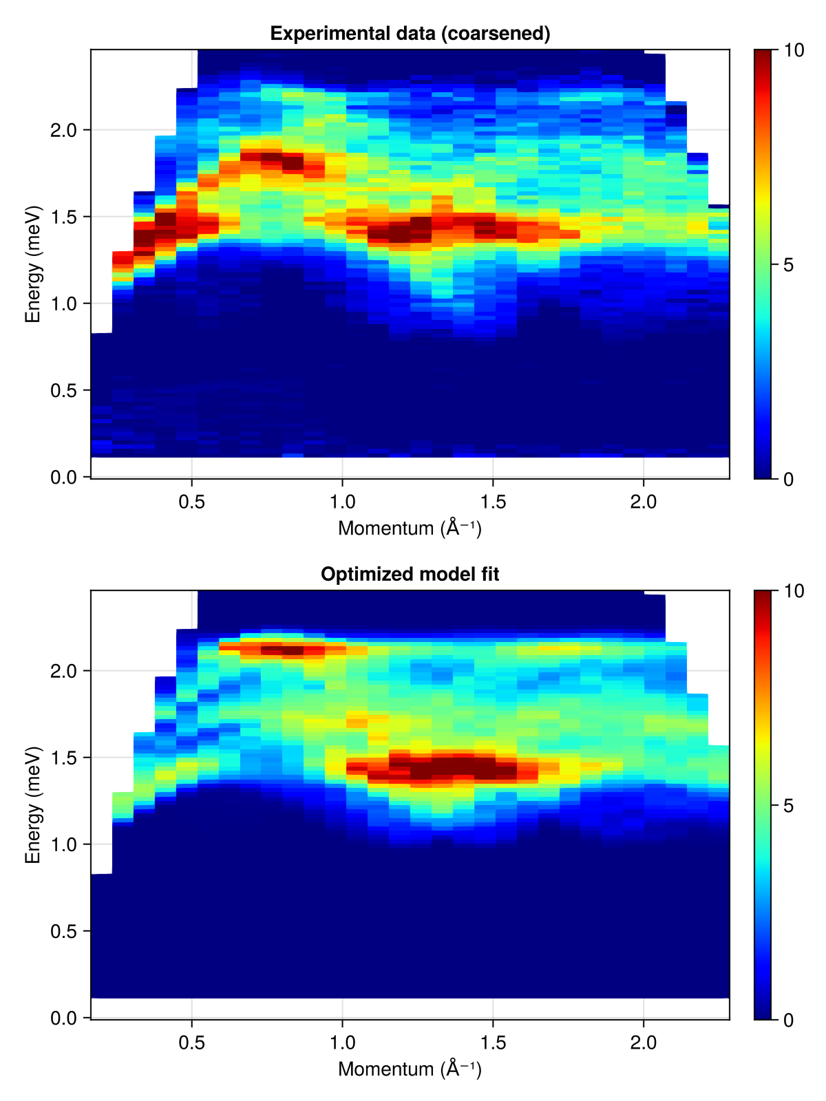
Finally, plot experimental and simulated intensities as they are seen by the loss function. The scale factor returned by squared_error_fitted allows to put both plots on the same global intensity scale.

set_params!(sys, labels, param_mapping(fit.minimizer))

minimize_energy!(sys)
swt = SpinWaveTheory(sys; measure)

res = powder_average(cryst, radii, 1000) do qs
    intensities(swt, qs; energies, kernel)
end

(; scale) = squared_error_fitted(ref_data, res.data; scale=true)

fig = Figure(; size=(600, 800))

res.data[findall(isnan, ref_data)] .= NaN
plot_intensities!(fig[2, 1], res; colormap=:jet1, colorrange=(0, 10.0),
                  title="Optimized model fit", units)

res.data .= ref_data * scale
plot_intensities!(fig[1, 1], res; colormap=:jet1, colorrange=(0, 10.0),
                  title="Experimental data (coarsened)", units)
fig